Accelerated Life Testing: Estimating Lifetime with the Arrhenius Model

Encoders are specified for a ten-year life, yet tests last only a few thousand hours. This article derives the acceleration-factor formula from reaction rates, shows with LED and adhesive examples how strongly activation energy affects AF, presents a simulated three-temperature test with extrapolated lifetime confidence intervals, and lists typical cases where the model breaks down.

An encoder’s LED light output decays with time, and the adhesive between the encoder disc and the hub ages as well. If continuous operation for 10 years (about 8.8×10⁴ h) is required, a real-time test of that length is impossible. The usual approach is to raise the temperature so that degradation accelerates, then convert the test time back to use conditions with a model. How large that conversion factor is—and whether it can be trusted—depends on understanding the Arrhenius model.

Figure 1 – When the test temperature rises from 40 ℃ to 105 ℃, the failure-time distribution shifts left as a whole on a log-time axis without changing shape; the shift is the acceleration factor AF (Ea = 0.7 eV, assumed)

From reaction rate to acceleration factor

Many degradation processes (diffusion, oxidation, chemical reaction) obey a rate of the form

R = A·exp(−Ea / (k·T))

where Ea is the activation energy (eV), k = 8.617×10⁻⁵ eV/K is Boltzmann’s constant, T is the thermodynamic temperature (K), and A is a temperature-independent constant.

If the change of a degradation measure D is written dD/dt = R(T)·g(D), with g describing the shape of the degradation curve, integrating to a failure criterion D_f gives G(D_f) = R·t_f, so the failure time t_f is inversely proportional to the rate. Provided g does not change with temperature, the ratio of failure times at the use temperature T_u and the stress temperature T_s is

AF = t_u / t_s = exp[(Ea/k)·(1/T_u − 1/T_s)]

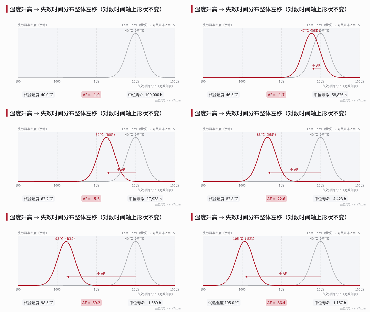
An important corollary follows: temperature simply compresses the time axis by a constant factor. On a log-time axis, therefore, failure distributions at different temperatures should translate without changing shape (Figure 1); when a lognormal or Weibull model is used, σ or the shape parameter should be the same. That is the first check that “the mechanism has not changed”.

Worked examples: LED and adhesive

LED, use at 40 ℃, test at 85 ℃, Ea taken as 0.7 eV (assumed):

1/T_u − 1/T_s = 1/313.15 − 1/358.15 = 4.012×10⁻⁴ K⁻¹ Ea/k = 0.7 / 8.617×10⁻⁵ = 8123 K AF = exp(8123 × 4.012×10⁻⁴) = exp(3.259) ≈ 26.0

So 1000 h at 85 ℃ is equivalent to about 2.6×10⁴ h at 40 ℃.

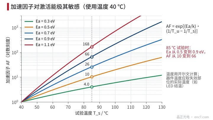
Activation energy has a huge effect (Figure 2): for the same 40→85 ℃ step, Ea = 0.3, 0.5, 0.7, 0.9, 1.1 eV give AF = 4.0, 10.3, 26.0, 66.1, 168 respectively. A 0.2 eV difference in Ea changes AF by a factor of about 2.5.

Figure 2 – At a use temperature of 40 ℃, acceleration factor versus test temperature and activation energy; at 85 ℃, as Ea goes from 0.5 to 0.9 eV, AF goes from 10 to 66

Temperature must also be the actual temperature of the failing site. Assume an LED dissipates 30 mW with a junction-to-ambient thermal resistance of 300 K/W; the junction is then about 9 K hotter than ambient. Using junction temperatures of 49 ℃ and 94 ℃ gives AF ≈ 22.0; using ambient temperatures directly overestimates AF by about 18%.

Adhesive, use at 60 ℃, test at 105 ℃: with Ea taken as 0.6, 0.8, 1.0 eV (assumed), AF = 12.0, 27.6, 63.1. Raising the test temperature further to 125 ℃ for more acceleration can push AF to 30~295. But if the glass-transition temperature Tg of that adhesive is about 110 ℃ (assumed), at 125 ℃ the adhesive leaves the glassy state for the rubbery state, creep, moisture uptake and reaction paths may all change, and that set of AF values loses meaning.

Where activation energy comes from

Ea is a parameter of a specific failure mechanism, not a material constant and not a device constant. There are three sources:

literature and industry data for the same mechanism; for common electronic-device mechanisms Ea is typically of the order of a few tenths to a little over one eV;
test data from the component or material supplier under the same failure criterion;
a multi-temperature test of your own. With two temperatures, Ea = k·ln(t₁/t₂) / (1/T₁ − 1/T₂).

When data are lacking, 0.7 eV is often taken as a default—but that is only a convention. Overestimating Ea overestimates AF and therefore lifetime; the conclusion is biased toward the unsafe side.

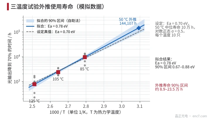
Figure 3 shows a simulated three-temperature test: true Ea = 0.70 eV, median life at 50 ℃ = 10×10⁴ h, lognormal σ = 0.5, 10 LEDs each at 85, 105 and 125 ℃, failure criterion light output down to 70%. Even when the data are generated exactly from the model, the fit yields Ea = 0.78 eV (90% interval 0.67~0.88 eV) and an extrapolated 50 ℃ median life of 14.4×10⁴ h with a 90% interval of about 8.9×10⁴~23.5×10⁴ h. The farther the extrapolation, the wider the interval.

Figure 3 – Arrhenius plot of a three-temperature test: the fitted line extrapolated to 50 ℃, with a shaded 90% bootstrap interval (simulated data)

When the model breaks down

Mechanism changes with temperature: above the adhesive’s Tg, or beyond the temperature rating of the LED encapsulant, failures appear that do not occur under use conditions.
Several mechanisms coexist: for two mechanisms with Ea of 0.4 and 1.0 eV, a high-temperature test mainly amplifies the high-Ea mechanism, while at use temperature the low-Ea mechanism may occur first—and the test has masked it.
Stresses other than temperature: humidity needs a Peck-type isothermal humidity model, temperature cycling needs a Coffin–Manson relation, and LED drive current itself affects lumen depreciation.
Censored data: tests often stop when only some samples have failed; a maximum-likelihood method that handles censoring should be used, not a simple average of the already-failed samples.

Engineering points

Convert every temperature to kelvin and use the temperature of the failing site: junction temperature for an LED, measured temperature for an adhesive layer; self-heating of 9 K can already bias AF by about 18%.
Run at least three temperatures and check that the distribution shape parameter is consistent across them; inconsistency means the mechanism has changed and extrapolation is invalid.
Keep the highest test temperature below material limits with margin: below Tg for adhesives, below the allowed junction temperature for LEDs.
When a reliable Ea is unavailable, take a low value and state the source in the report; every 0.2 eV overestimate of Ea overestimates lifetime conversion from an 85 ℃ test by a factor of about 2.5.
Define the failure criterion by encoder function—for example light output so low that automatic gain can no longer compensate, or signal amplitude below its lower limit—not a blanket “70%”.
Report lifetime with a confidence interval and the extrapolation distance, not as a single number.

Summary

Arrhenius acceleration is temperature compressing the time axis by a constant factor, AF = exp[(Ea/k)·(1/T_u − 1/T_s)]. Its credibility rests almost entirely on whether Ea corresponds to a real single failure mechanism and whether that mechanism stays the same at high temperature. Checking shape consistency across multi-temperature tests and reporting confidence intervals is what makes accelerated-test conclusions stand up.

Translated from the ENC7 Chinese technical library (article 0193). Read the Chinese original. Need a disc built to your drawing? Request a quote or see our custom encoder discs.