Industry applications in depth
AGV Drive-Wheel Odometry: Diameter, Line Count, Dead-Reckoning Error
Differential-drive AGVs perform dead reckoning with the drive-wheel encoders. This article computes a resolution of 5.89 μm for a 150 mm wheel diameter, a reduction ratio of 20 and a 1000-line encoder, compares the disparity between quantization error (0.24 mm at 10 m) and a 0.5% wheel-diameter difference (0.5 m), and gives a reasonable resolution range and the calibration priorities.
Dead reckoning on a differential-drive AGV uses only the encoders on the two drive wheels: in each sampling period the displacements of the left and right wheels are taken, and the heading change is obtained from their difference. A question often arises when selecting the encoder: the higher the motor-encoder line count, the more accurate the odometry? Once the errors are separated by source, the answer is no.
The model: how heading error becomes lateral deviation
Let the left- and right-wheel displacement increments be Δs_L and Δs_R, and the wheelbase be b. Then
Δs = (Δs_R + Δs_L)/2,Δψ = (Δs_R − Δs_L)/b
where Δs is the advance of the vehicle body and Δψ is the heading change. For every subsequent advance s, a heading error ψ_err adds a lateral deviation of ψ_err·s. The two classes of error behave differently:
- Bounded error: encoder quantization. The count is a cumulative quantity and is not lost; the cumulative displacement error of each wheel never exceeds ±1 count, the heading error is bounded, and the lateral deviation grows only linearly with distance.
- Accumulating error: the distance travelled per revolution differs between the two wheels, for example because of a wheel-diameter difference or an error in the effective wheelbase. The heading error itself grows with distance, and the lateral deviation grows with the square of distance.
Quantization error: a resolution of 5.89 μm
Worked example: wheel diameter 150 mm (circumference 471.2 mm), reduction ratio 20, a 1000-line motor encoder with fourfold decoding. Then
counts per wheel revolution = 4000 × 20 = 80 000,per count = 471.2 mm ÷ 80 000 = 5.89 μm
Each of the two wheels has a deviation of ±1 count. Taking the wheelbase as 0.5 m, the upper bound on heading error is Δψ = 2 × 5.89 μm ÷ 0.5 m = 2.36×10⁻⁵ rad (4.9″). After 10 m of straight travel the upper bound on lateral deviation is 2.36×10⁻⁵ × 10 m = 0.24 mm.
Wheel-diameter difference: quadratic growth
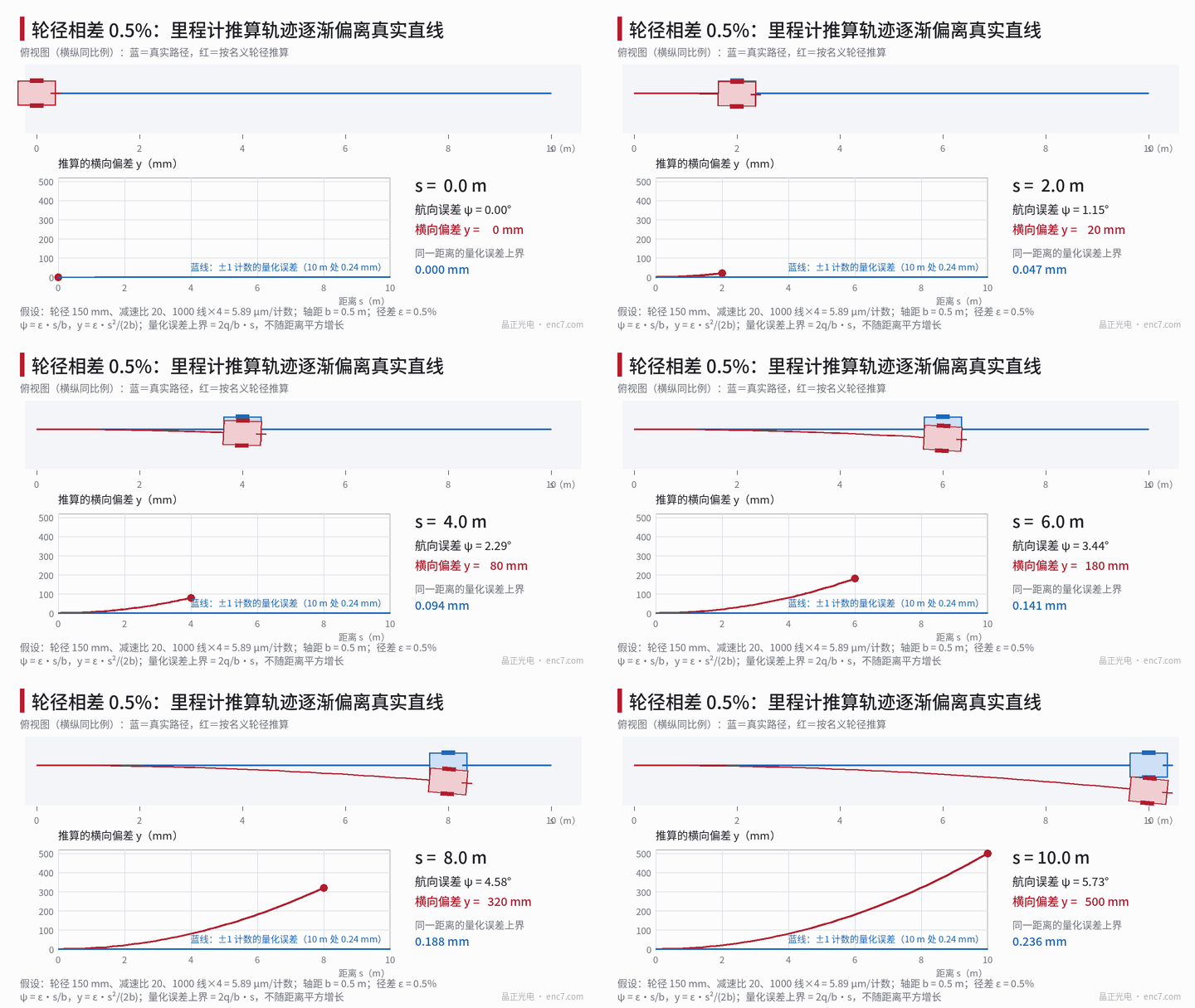
When the two wheel diameters differ by ε, if the true path is a straight line the two wheels actually roll the same distance, whereas the estimate that uses the nominal diameters gives a left–right path difference of ε·s, so
ψ(s) = ε·s/b,y(s) = ε·s²/(2b)
where y is the lateral deviation of the estimated position from the true path. For ε = 0.5% (a diameter difference of about 0.75 mm on a 150 mm wheel, for example from uneven wear) and b = 0.5 m, at 10 m one has ψ = 0.1 rad (5.7°) and y = 0.5 m. Conversely, if the two wheels are controlled to the same count on the basis of the nominal diameters, the true path bends into a circular arc of radius b/ε = 100 m, and the deviation has the same magnitude. For b = 0.5 m, y = ε·s²:
| ε \ s | 2 m | 5 m | 10 m | 20 m |
|---|---|---|---|---|
| 0.1% | 4 mm | 25 mm | 100 mm | 400 mm |
| 0.5% | 20 mm | 125 mm | 500 mm | 2000 mm |
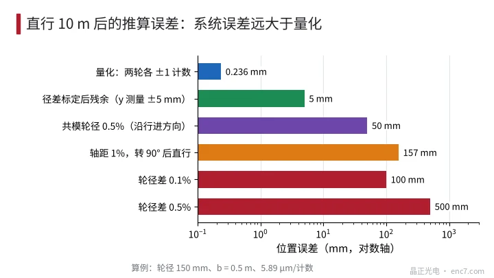
The magnitudes of the various errors at 10 m are shown in Figure 2. A 0.5% diameter difference is about 2100 times the quantization error; if the effective wheelbase is off by 1%, after a 90° turn the heading is high by 0.9°, and 10 m of straight travel then deviates by 157 mm; if both wheels are simultaneously 0.5% undersize, heading is unaffected and only a 50 mm distance error appears in the direction of travel.
A reasonable range for the resolution
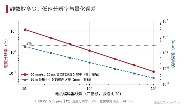
The lower bound on resolution is set by low-speed measurement, not by the odometry. Taking a minimum travel speed of 50 mm/s and a speed-measurement window of 10 ms, the number of counts traversed in the window is 0.05 × 0.01 ÷ 5.89 μm = 85, and the speed resolution is about 1.2%. If a figure of not less than 2% is required (at least 50 counts), each count must be no greater than 10 μm, that is not fewer than 47 100 counts per wheel revolution, which corresponds to about 590 lines or more for an encoder with fourfold decoding and a reduction ratio of 20. At 1000 lines the figure is 1.2%, at 500 lines 2.4% (Figure 3).
The upper bound has no meaning: even if the line count is raised further and the lateral error due to quantization falls from 0.24 mm to 0.02 mm, that has no effect against a systematic deviation of 0.5 m. If the motor already uses a 17–23 bit encoder, it can be used as it is; there is no need to raise the resolution specially for the odometry. At still lower speeds, switching to a pulse-interval method (the M/T method) can improve the speed resolution without increasing the line count.
Calibration priorities
- Wheel-diameter difference: let the AGV travel 10 m straight without heading correction, measure the lateral deviation y of the actual path from a straight line, then ε = 2·b·y/s². A heading error at the start will introduce a linear term, so a quadratic fit at several distance points is advisable. When the measurement error in y is ±5 mm, the uncertainty in ε is 2 × 0.5 × 0.005 ÷ 100 = 0.005%. After calibration, the residual deviation over a distance s is about ±5 mm × (s/10 m)².
- Effective wheelbase: rotate on the spot through several revolutions, measure the actual rotation with an external reference (for example a fixed target) and compare it with the estimated rotation to obtain a correction factor.
- Change with time: the diameter of polyurethane wheels changes with wear, load and temperature; they should be recalibrated periodically, or a gyroscope should be used to supply the heading and to estimate the diameter difference online.
- Slip: the encoder is on the motor side, so slip and tread creep are invisible; periodic correction with landmarks or laser localization is required.
Engineering points
- First compute the order of magnitude of each error source: quantization 0.24 mm, a 0.5% wheel-diameter difference already 0.5 m — the latter is what should be improved.
- A resolution of 5–10 μm per count is already sufficient for odometry; 1000 lines and 5.89 μm/count is a reasonable starting point.
- The lower bound on line count is set by requiring at least 50 counts in the speed-measurement window at the lowest speed, about 590 lines (reduction ratio 20, fourfold decoding).
- Calibrate the diameter difference from the lateral deviation of a 10 m straight run: ε = 2·b·y/s²; a measurement accuracy of ±5 mm corresponds to 0.005%.
- Fit left and right wheels from the same batch and in the same wear condition, and recheck the diameter difference periodically; a difference of 0.1% already gives a 100 mm deviation at 10 m.
- Odometry only covers relative position over short times; over long distances, correction comes from a gyroscope or from landmarks.
In brief
Error in drive-wheel odometry is dominated by systematic terms: quantization is bounded and is only 0.24 mm at 10 m; a wheel-diameter difference makes the lateral deviation grow with the square of distance, and 0.5% is already 0.5 m. An encoder resolution of 5–10 μm/count is already enough; a high line count will not improve the odometry. What is worth investing in is calibration of the diameter difference and the wheelbase, and periodic correction with a gyroscope or landmarks.
Translated from the ENC7 Chinese technical library (article 0766). Read the Chinese original. Need a disc built to your drawing? Request a quote or see our custom encoder discs.
© Langfang Jingzheng Optoelectronic Technology Co., Ltd. All rights reserved. This article was created with AI assistance.