Encoder-disc terminology
Averaging Effect: How Error Shrinks When the Detection Window Covers N Lines

The phase out of the readhead is a weighted average of the line positions inside the detection window. This article derives the 1/√N_eff shrinkage of random error and the sinc transfer of periodic error, computes the attenuation of a 2 mm window for different spatial periods, and shows with a worked example why a peak-to-peak graduation error of 14″ falls to about 4″ at the readhead—and how to align the specification basis when comparing figures.
A factory report quotes a peak-to-peak graduation error of 14″ measured line by line; after the disc is fitted into an encoder and calibrated on a rotary table, only about 4″ remain once eccentricity is removed. Neither side has measured wrongly: at every instant the readhead sees the composite signal of several tens of lines inside the detection window, and its phase is the weighted average of those line positions. Averaging suppresses random and short-period errors, but it is almost useless against long-period errors. This article writes that averaging effect as a transfer function and shows how much each class of error is attenuated.
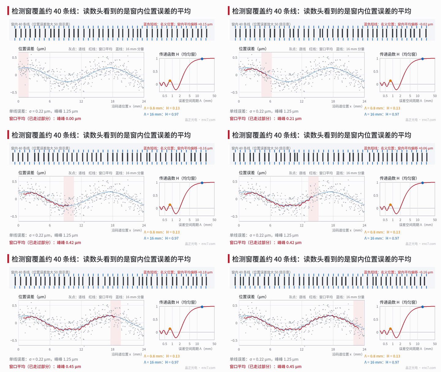
Definition: the readhead output is a weighted average over the window
Let the nominal position of line n be n·p and its actual deviation δ_n, and let the detection window weight on line n be w_n (the product of illumination intensity, detector response and index-grating transmittance). The fundamental out of the readhead is the sum of the line contributions:
S(x) = Σ w_n·cos[2π(x − n·p − δ_n)/p]
When δ_n is much smaller than p/(2π), the phase offset of the composite signal linearises to
ε(x) = Σ w_n·δ_n / Σ w_n
So the position error sensed by the readhead is the sliding weighted average (convolution) of the line-by-line error sequence with the normalised window weights. Worked example below: read radius r = 20 mm, 2500 lines (p = 50.3 μm), detection window length along the measuring direction L ≈ 2 mm, about 40 lines.
Random error: shrinks as 1/√N_eff
If the line errors are independent with standard deviation σ, the standard deviation after weighted averaging is
σ_ε = σ·√(Σw_n²) / Σw_n = σ / √N_eff, N_eff = (Σw_n)² / Σw_n²
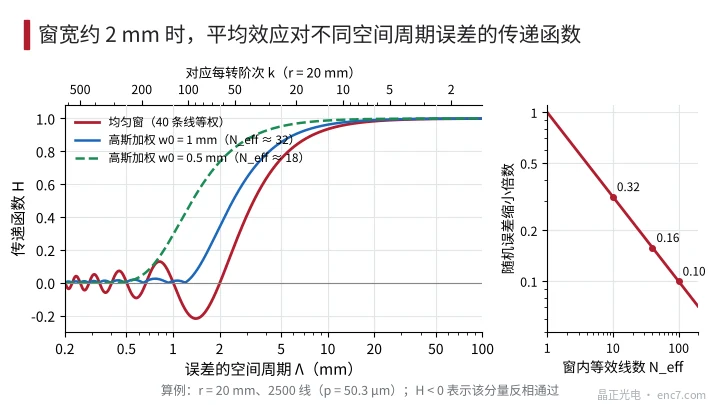
N_eff is the effective line count. Under uniform illumination N_eff equals the number of lines in the window N_w; under non-uniform illumination N_eff is smaller: for Gaussian illumination with a 1/e² radius of 1 mm truncated by a 2 mm window, N_eff ≈ 32; at a radius of 0.5 mm it is only about 18.
Worked example: σ = 0.2 μm (about 2.06″ at r = 20 mm) becomes 0.032 μm, about 0.33″, after a uniform 40-line window. If neighbouring lines are correlated—for example through a long-period component from the same writing process—the √N rule no longer applies and the transfer function below must be used.
Periodic error: a sinc-type transfer function
A sinusoidal component of spatial period Λ (length along the track) in the line-by-line error is multiplied, after a uniform window, by
H(Λ) = sin(πN_w·p/Λ) / (N_w·sin(πp/Λ)) ≈ sinc(L/Λ), sinc(u) = sin(πu)/(πu)
where L = N_w·p is the window length. Written as orders per revolution k = 2πr/Λ, this is the sliding-average formula of the error-spectrum-decomposition article in this library. Several features:
- when Λ = L/m (m an integer), H = 0 and that component is completely averaged out;
- near Λ ≈ 0.70L there is a sidelobe of about −0.217, the minus sign meaning the component passes with inverted phase;
- when Λ is much smaller than L, |H| does not exceed Λ/(πL);
- when Λ > 5L, H > 0.93 and there is almost no attenuation.
Numerical values for L = 2 mm, r = 20 mm:
| Spatial period Λ | Order per rev. k | Uniform-window H | Gaussian-weighted H (1/e² radius 1 mm) |
|---|---|---|---|
| 62.8 mm | 2 | 0.998 | 0.999 |
| 10 mm | 12.6 | 0.935 | 0.962 |
| 4 mm | 31 | 0.637 | 0.782 |
| 2 mm | 63 | 0 | 0.339 |
| 1.33 mm | 94 | −0.212 | 0.040 |
| 0.8 mm | 157 | 0.127 | 0.023 |
A uniform window has zeros and sidelobes; Gaussian weighting has no zeros, suppresses high frequencies more thoroughly, but reduces N_eff and weakens the attenuation of mid-period components (see Figure 2).
Why line-by-line graduation error exceeds what the readhead senses
Figure 3 is an example: the line-by-line error is composed of random σ = 0.15 μm, a 3rd-order 0.15 μm and a 150th-order 0.10 μm (Λ ≈ 0.84 mm).
| Component | Line-by-line peak-to-peak | Peak-to-peak after 40-line window average |
|---|---|---|
| Random | 11.2″ | 1.2″ |
| 150th order | 2.1″ | 0.26″ |
| 3rd order | 3.1″ | 3.1″ |
| Total | 14.0″ | 4.1″ |
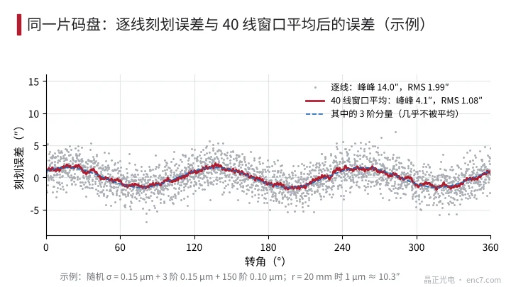
The difference comes from three places: the RMS of the random component shrinks by √40, while the peak-to-peak of the line-by-line data is about 7σ and after averaging neighbouring points are highly correlated so the peak-to-peak is only about 5σ—hence a peak-to-peak shrinkage of about 9.5×, more than √40; short-period components are attenuated by H; and the repeatability of the line-by-line measuring instrument itself is mixed into the single-line error, whereas the readhead does not see that term. Conversely, long-period components are as large in the line-by-line measurement as at the readhead; eccentricity, clamping deformation and other low-order errors cannot rely on averaging.
Window size also sets the sensitivity to short-period error. On the same disc with a small readhead of window length about 0.5 mm (10 lines), random error shrinks only to 0.32× and the 0.84 mm-period component still retains about 51%. The same disc can therefore show different accuracy on different readheads for exactly this reason.
A larger window is not always better either: the longer the window, the more sensitive the readhead becomes to radial displacement, azimuth and disc flatness (see the cross-sensitivity and azimuth-alignment articles in this library). When the A and B detection fields are laid out separately, each channel averages a different set of lines, and an error whose spatial period matches the field spacing appears as A/B phase ripple.
Engineering points
- State whether a graduation-error specification is single-line or an N-line window average, and give the window length and weight shape; otherwise the numbers cannot be compared.
- Before comparing line-by-line data with encoder calibration results, apply the readhead window weights as a sliding weighted average to the line-by-line data.
- Random error shrinks as 1/√N_eff; N_eff is set by the illumination and detection weights and under Gaussian illumination is clearly smaller than the number of lines in the window.
- Errors with Λ > 5L are almost not averaged; eccentricity, clamping and low-order graduation errors must be controlled by process and centring.
- A uniform window has an inverted sidelobe of about 21% near Λ ≈ 0.7L; if a writing or stitching error of a particular period exists, check whether it falls exactly on that sidelobe.
- When selecting a disc, evaluate graduation error against the actual readhead window; small-window readheads are more sensitive to short-period error.
Summary
The phase out of the readhead is a weighted average of the line positions inside the window: random error shrinks as 1/√N_eff, periodic error is transferred by sinc(L/Λ), and errors whose period is much longer than the window are almost unaffected. Line-by-line graduation error includes the random and short-period components that are averaged away, plus measurement noise, so it is usually larger than what the readhead actually senses. Write the window basis into the specification and process the line-by-line data with the same window, and the two sides’ numbers will match.
Translated from the ENC7 Chinese technical library (article 0264). Read the Chinese original. Need a disc built to your drawing? Request a quote or see our custom encoder discs.
© Langfang Jingzheng Optoelectronic Technology Co., Ltd. All rights reserved. This article was created with AI assistance.