Competing technologies and trends
Cameras and pattern recognition: computational-imaging position measurement
Shooting a coded pattern or a random texture with an image sensor, then decoding for absolute position and using image correlation for sub-pixel translation, is a measuring approach still under development. This article derives a noise floor for sub-pixel estimation, compares the systematic bias of three fitting methods in simulation, and quantifies the constraints of motion blur, frame rate, latency and computing load.
A conventional encoder reads a carefully designed graduation with a few photodiodes, and the signal processing is done in the analogue domain. Another idea is to photograph a patch of pattern with an image sensor and leave decoding and registration to an algorithm. A familiar everyday example is the optical mouse, which images the desk texture at several thousand frames per second and estimates displacement by correlation. If this idea is turned into precision position measurement, how accurate and how fast can it be, and where is the cost?
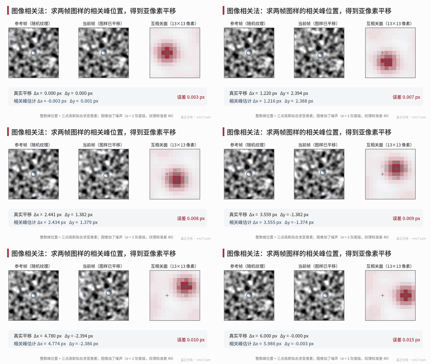
Principle: decoding gives the absolute position, registration the fine position
Computational-imaging measurement usually has two layers:
- Coarse positioning (absolute): the pattern is a two-dimensional pseudo-random code or a marked code array, and the combination in any k×k window does not repeat over the full measuring range. A binary 6×6 window has 2³⁶ combinations, far more than the number of positions actually needed, and the surplus can be used for error correction. Decoding the code word shows which code element the centre of the field of view lies in.
- Fine positioning (sub-pixel): inside the code element, the current frame is registered to a reference pattern to obtain the translation.
Registration commonly uses cross-correlation: c(u, v) = Σ I₁(x, y)·I₂(x + u, y + v), and the peak location is the translation. Computed with an FFT, c = F⁻¹[F(I₁)*·F(I₂)]; if the spectral magnitude is normalized and only the phase is kept, the method is phase correlation. Beyond the integer peak location, a parabola or a Gaussian is fitted to the three points around the peak to obtain the sub-pixel offset, or a gradient iteration method (Lucas–Kanade) is used to solve for the translation directly.
The object-side resolution is set by the pixel size and the magnification: with a 3.45 μm pixel and a magnification of 1, each object-side pixel is 3.45 μm; if the sub-pixel accuracy reaches 0.01 pixel, that corresponds to 34.5 nm, or about 0.36″ on an encoder disc of 20 mm radius.
Noise floor: the Cramér–Rao bound
Assume the reference pattern is noiseless and each pixel of the current frame has independent noise of variance σ_n². The lower bound on the variance of the translation estimate along x is
σ_δ² ≥ σ_n² / Σ(∂I/∂x)²
where the sum runs over all pixels used in the registration. This says two things: the steeper the texture gradient and the more pixels there are, the higher the accuracy; the noise falls as 1/√(pixel count). Worked example: 128×128 pixels, RMS texture grey-level gradient 25 grey levels/pixel, noise 2 grey levels, σ_δ ≥ 2/(128×25) ≈ 6×10⁻⁴ pixel. In simulation the random error of the gradient iteration method is about 8×10⁻⁴ pixel, of the same order as the bound. If the reference frame also contains noise, the bound is multiplied by about √2.
Systematic bias: pixel locking
Random error can be averaged out; systematic bias cannot. A three-point fit assumes that the peak shape is a parabola or a Gaussian, whereas the actual peak shape depends on the texture, so the estimate is “pulled” toward integer pixels and the error follows an S-shaped curve with the true sub-pixel position — this is called pixel locking.
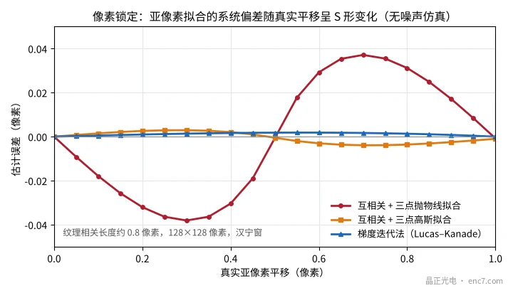
The simulation conditions are a texture correlation length of about 0.8 pixel, 128×128 pixels, and a Hanning window. The bias of the three-point parabolic fit is about 0.038 pixel at most, that of the Gaussian fit about 0.004 pixel, and that of gradient iteration about 0.002 pixel. The situation worsens when the texture is too fine: if the correlation length drops to 0.5 pixel the pattern is undersampled, and the bias of the gradient method also rises to about 0.03 pixel. Pattern features should therefore cover at least two pixels.
A real system also has systematic errors from lens distortion, uneven illumination, pixel response non-uniformity, and magnification change with temperature. The few-thousandths of a pixel seen in an ideal simulation are often out of reach in practice; holding a stable accuracy of the order of one hundredth of a pixel already takes careful calibration.
Speed, latency and computing load
Motion blur: during the exposure the pattern moves by v·t_exp. With 1 μs pulsed illumination, the blur at 1 m/s is 1 μm, about 0.29 pixel, which is still acceptable; with a 10 μs exposure it becomes 2.9 pixels.
Frame-to-frame displacement: when only relative registration is used, adjacent frames must overlap enough. With a 128-pixel field of view (about 0.44 mm), if the frame-to-frame displacement is required not to exceed 1/4 of the field of view, the speed limit at a 10 kHz frame rate is about 1.1 m/s. An absolute pattern that can be decoded independently in every frame does not have this restriction.
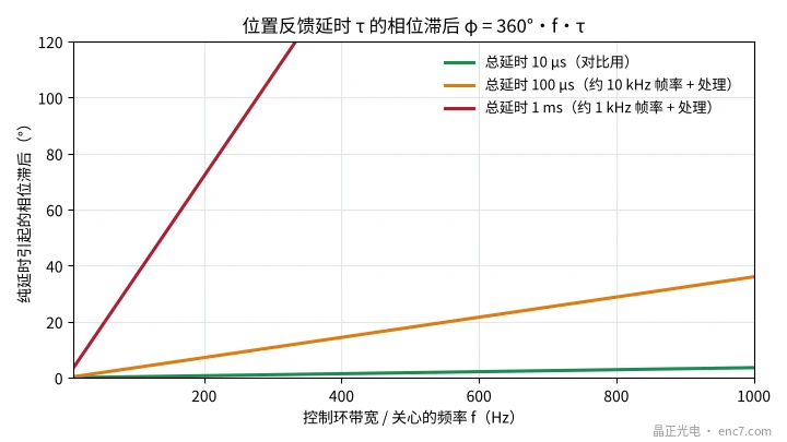
Latency: exposure, readout and computation add up to a total latency τ, which produces a phase lag of 360°·f·τ at frequency f. With τ = 100 μs the lag is 7.2° at 200 Hz and 36° at 1 kHz, which cannot be ignored in a high-bandwidth servo loop (see Figure 3).
Computing load: a 128×128 complex FFT takes about 5N·log₂N ≈ 1.1×10⁶ floating-point operations; each frame needs at least one forward and one inverse transform, so at a 10 kHz frame rate that is about 2×10¹⁰ operations per second, with a data rate of about 164 MB/s. This usually requires an FPGA or dedicated hardware.
Frontier directions and practical difficulties
- The pattern is still the reference: the camera measures the position of “the pattern relative to the sensor”; a position error Δx of the pattern itself becomes an angular error Δθ = Δx/r directly. Precision measurement still needs lithographic accuracy in the pattern; a random texture needs point-by-point calibration and then faces drift from wear and contamination.
- Multiple degrees of freedom: a single image can solve for x, y and rotation together, which suits multi-axis stages and is a distinctive advantage over a one-dimensional encoder.
- Combination with grating interpolation: the camera handles absolute position and high accuracy at low speed, while a conventional grating readhead provides high-speed, low-latency continuous interpolation — a possible hybrid architecture.
- New sensors and algorithms: event-based vision sensors and learning-based decoding are under study, but calibration, interpretability and long-term stability still need to be demonstrated.
Engineering points
- Work out the object-side pixel first: pixel size ÷ magnification, then multiply by the achievable sub-pixel accuracy (in practice estimate on the order of 0.01 pixel) to obtain the resolution that can be counted on.
- Choose the right sub-pixel method: pixel locking of a three-point parabolic fit can reach several hundredths of a pixel; for precision work use a Gaussian fit, a phase method or gradient iteration.
- Pattern features no smaller than 2 pixels: undersampling increases the bias of every method.
- Use pulsed illumination to hold down blur: keep the blur v·t_exp within a few tenths of a pixel.
- Check the effect of latency on the control loop: φ = 360°·f·τ; 100 μs of latency is already 36° at 1 kHz.
- Put pattern accuracy into the error budget: a camera scheme does not remove the need for a high-accuracy pattern; pattern position error enters the measurement directly.
Summary
Computational-imaging measurement replaces “graduations + analogue interpolation” with “take a picture + run an algorithm”, and is attractive for multiple degrees of freedom, absolute positioning and error tolerance. The theoretical floor on sub-pixel accuracy can be very low, but pixel locking, systematic errors from the lens and the illumination, frame rate and latency, and computing load are the practical constraints. It is more likely to complement a conventional grating readhead than simply to replace it, and the precision pattern itself remains the measuring reference.
Translated from the ENC7 Chinese technical library (article 0187). Read the Chinese original. Need a disc built to your drawing? Request a quote or see our custom encoder discs.
© Langfang Jingzheng Optoelectronic Technology Co., Ltd. All rights reserved. This article was created with AI assistance.