Testing, reliability & quality
Deep Learning for Encoder-Disc Visual Inspection: What It Can Do and What to Watch
Rule-based AOI never misses dimensional defects but is often flooded by pseudo-defects such as particles and stains; deep learning is good at separating appearance classes but depends on samples and thresholds. This article compares the two scopes of use, shows with simulated data the trade-off of threshold, overkill and escape and a cost-optimal threshold, and calculates how many defective samples are needed to verify an escape rate.
Encoder-disc visual inspection looks for a mixed bag of defects: chrome pinholes, residual-chrome bridges, broken lines, scratches, particles, edge chips, stains. Rule-based AOI can compare the image with the design pixel by pixel and is reliable on dimensional decisions, but it is sensitive to “different” and dull to “whether different matters”; one disc may throw dozens of candidates, most of them dust and harmless edge undulation, and a human recheck finishes the job. Deep learning seems to fill exactly that gap—but it turns the problem from “tuning parameters” into “managing data and thresholds”.
What rule-based AOI and deep learning each do well
| Dimension | Rule-based AOI | Deep learning |
|---|---|---|
| Principle | Compare with design or gold sample, thresholds, morphology, dimensional measurement | Learn defect features from labelled samples; output class or pixel-level segmentation |
| Samples needed | Essentially no defective samples | Enough representative labelled samples |
| Dimensional decisions | Strong; uncertainty evaluation possible | Weak; not suited as a direct measurement |
| Appearance decisions | Weak; many pseudo-defects | Strong; can separate particles and stains from true defects |
| Illumination / process drift | Sensitive; repeated retuning | Fairly robust to variations covered by the training set; uncovered ones may fail |
| Interpretability and traceability | Rules are explicit | Needs heat maps and similar aids; conclusions depend on data version |
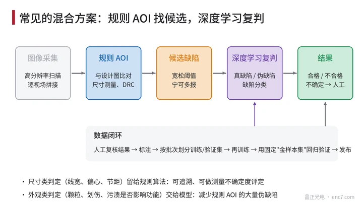
So a common practice is a hybrid (Figure 3): rule-based AOI with a loose threshold finds every candidate and finishes dimensional decisions; deep learning only rejudges and classifies candidates as “true defect or pseudo-defect”, and doubtful ones go to a human. With good samples only, an anomaly-detection model can also do a first screen—but it can only answer “does it look like a good part?”, not the defect type.
Images and samples: count the data volume first
Resolution is set by the smallest defect: a defect should occupy at least about 3 pixels on the image, so a 5 μm pinhole needs a pixel scale no coarser than about 1.7 μm. For a track zone of inner/outer radii 14 mm and 20 mm the area is about 641 mm²; a 1200×10⁴-pixel camera at 1.5 μm/pixel covers about 27.6 mm² per field of view, so one disc needs about 23 fields, or about 28 with overlap.
The hard part of sampling is that defects are rare and of many classes. Principles that must be obeyed:
- Split train and validation by batch. If images from the same disc or the same batch appear in both train and validation, validation scores are inflated.
- Define labelling rules first: how large a pinhole counts as a defect, whether a particle on a chrome line counts—write the acceptance standard, then label; when several people label, measure agreement and discuss disputed samples separately.
- Cover process variation: different coating batches, different illumination ageing states and different disc designs must appear in the training set; a new design needs re-validation before release.
Confusion matrix and threshold
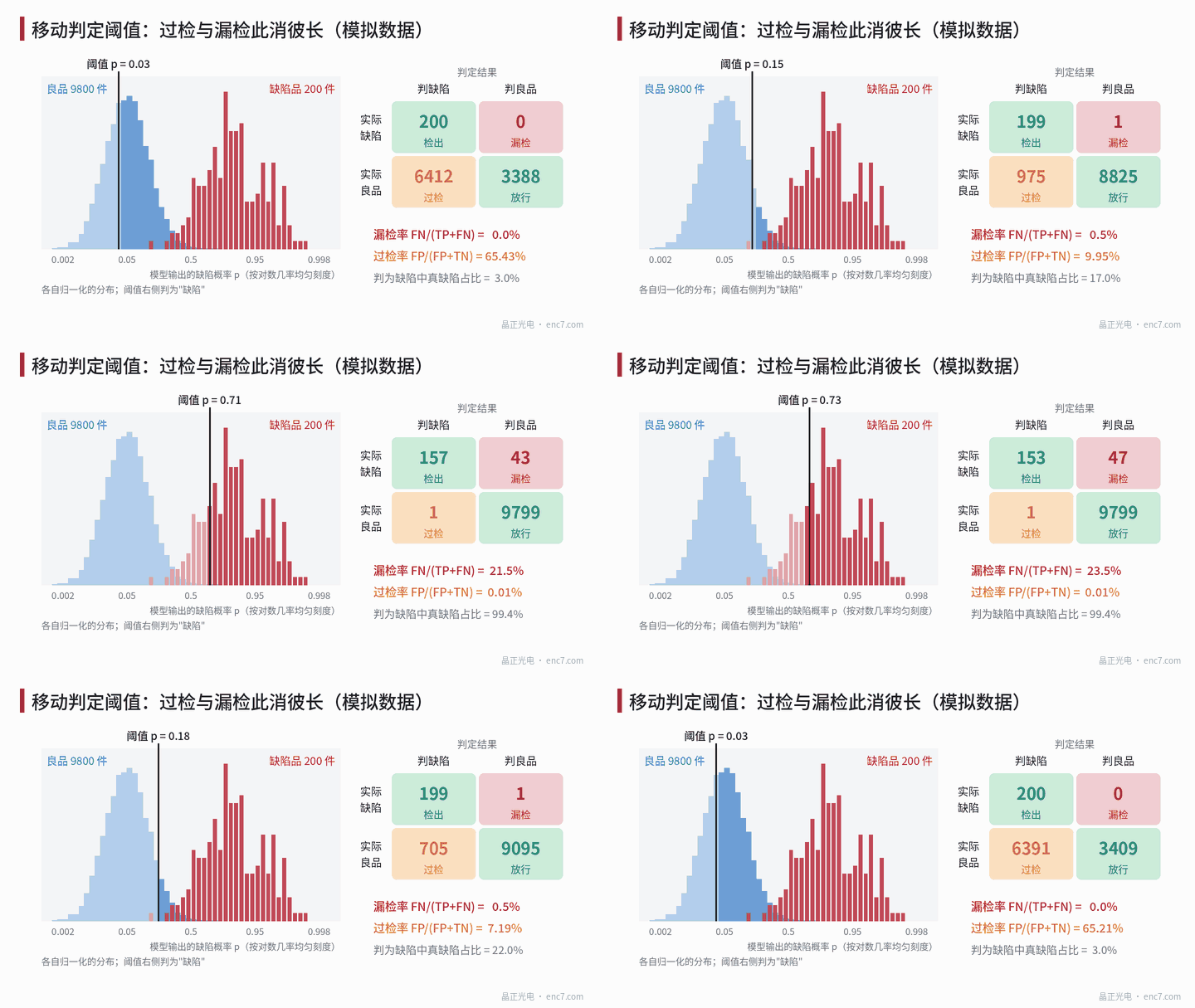
The model outputs a defect probability p for each candidate; above the threshold it is called a defect. Four outcomes form the confusion matrix: detection (TP), escape (FN), overkill (FP), pass (TN). Common metrics:
escape rate = FN / (TP + FN), overkill rate = FP / (FP + TN)
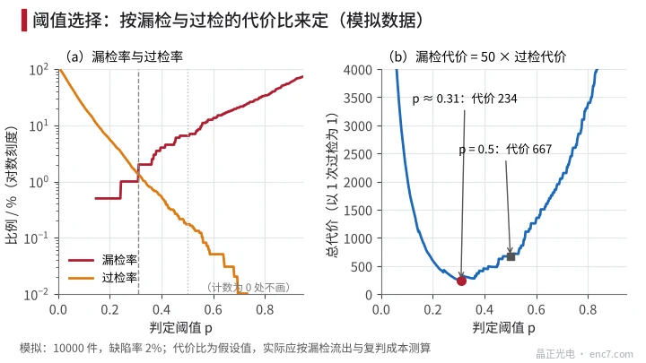
Example (simulated data, 10000 pieces, 2% defect rate): at threshold 0.5, 13 escapes (6.5%), 17 overkills (0.17%), and true defects are 91.7% of pieces called defective. At threshold 0.31, escapes fall to 2 (1.0%) and overkills rise to 134 (1.37%).
The threshold should be chosen by cost. Suppose the cost of one escaped defect reaching the field is 50 times the cost of one overkill (an extra recheck or a false scrap) (assumed); total cost = 50·FN + FP is minimum at about threshold 0.31 in this example, equal to 234, versus 667 at the default 0.5 (Figure 2). 0.5 is only the mathematical midpoint, not an engineering optimum.
Also watch the base-rate effect of a low defect rate: at only 2% defects, even an overkill rate of 1.37% means about four tenths of pieces called defective are still good. That is exactly why a human recheck channel must be kept.
How many samples to prove an escape rate
The figure “2 escapes / 200 = 1.0%” itself has statistical uncertainty; under a binomial distribution the 95% upper confidence bound is about 3.1%. To prove that the escape rate is no higher than p with zero escapes in the verification, the number of defective samples needed is
n ≥ ln(1 − CL) / ln(1 − p)
At confidence CL = 95% and p = 1%, n ≈ 299; at p = 0.5% about 598; if 1 escape is allowed, p = 1% needs about 473. For a product such as an encoder disc with a very low defect rate, accumulating a few hundred real defective samples often takes a long time—the most practical bottleneck before deep-learning inspection goes live.
Engineering points
- Leave dimensional decisions to rule algorithms; let deep learning only rejudge appearance—preserving measurement traceability while cutting pseudo-defects.
- Set the threshold by “escape cost ÷ overkill cost” and plot overkill and escape versus threshold on the validation set; do not default to 0.5.
- Verifying an escape rate needs at least about 3/p defective samples with zero escapes; when samples are short, report the upper confidence bound honestly.
- Split train and validation by batch; never let images of the same disc cross sets.
- Keep a fixed gold-sample set (including boundary defects of every class) and re-run regression after every model update or camera/light change.
- After go-live, monitor drift of the score distribution; an upward shift of good-part scores often appears before the overkill rate rises and signals illumination ageing or process change.
Summary
The value of deep learning in encoder-disc visual inspection is mainly to filter the flood of pseudo-defects from rule-based AOI, not to replace dimensional measurement. Its performance is set by samples, labels and threshold: choose the threshold by cost, prove the escape rate with enough defective samples, and keep validating the model across batches and process changes. Treat it as a measurement system that needs management, not as a black box, and it will stay reliable.
Translated from the ENC7 Chinese technical library (article 0199). Read the Chinese original. Need a disc built to your drawing? Request a quote or see our custom encoder discs.
© Langfang Jingzheng Optoelectronic Technology Co., Ltd. All rights reserved. This article was created with AI assistance.