Encoder-disc terminology
Error Statistics: Peak-to-Peak, ± Values, RMS and 2σ Conversion
Report the same error curve as peak-to-peak, ± value, RMS or 2σ and the numbers can differ by a factor of 2–4. This article derives PV = 2√2·RMS for a sine and PV = 2√3·σ for a uniform distribution, gives the d₂(n) table showing how the peak-to-peak of Gaussian error grows with sample count, explains that root-sum-square applies only to RMS-type quantities, and lists five common misjudgements.
The supplier’s report says “error RMS 3.5″”, the customer’s specification is “±5″”, and there seems to be plenty of margin; the customer re-measures, gets a peak-to-peak value of 9.9″ and declares the part out of tolerance. Neither data set is wrong; the mistake is comparing different statistics directly. There is no fixed ratio between the peak-to-peak, ± value, RMS and 2σ of an error curve; the ratio depends on the shape of the curve and on the number of samples. This article gives the conversions between these quantities and which one to use for combining and comparing.
Definitions: what each quantity measures
For an error record e_1 … e_n:
- Peak-to-peak PV = max e − min e, independent of the choice of zero.
- ± value has two definitions: ±PV/2 (zero at the midpoint of maximum and minimum), or the maximum absolute deviation from a specified zero, max|e − e_0|. When the curve is asymmetric or the zero is not at the midpoint, the latter is larger (for the influence of the zero choice see the graduation-error article in this library).
- RMS = √(Σe²/n), referred to zero; standard deviation σ = √(Σ(e − ē)²/n), referred to the mean. They satisfy RMS² = ē² + σ². The zero of an angular error is a convention in the first place, so before reporting RMS, state whether the mean has been removed; otherwise RMS changes with the zero.
- 2σ is twice the standard deviation, normally used as the half-width of a ± interval, i.e. ±2σ with a full width of 4σ. Some people also write the full width of the ±σ interval as “2σ”; the two readings differ by a factor of two.
Shape factors: deterministic curves and random error
First convert every quantity to σ (with zero mean, σ = RMS).
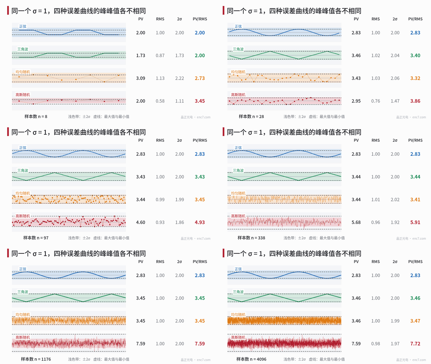
Sine e = A·sinθ: σ = A/√2 and PV = 2A, so
PV = 2√2·σ ≈ 2.83σ, 2σ = √2·A ≈ 0.71·PV
The values of a sine are concentrated at the two ends (arcsine distribution). ±2σ = ±1.41A already exceeds the maximum of the curve, so all samples lie inside the interval; its 95% interval is ±0.997A, about ±1.41σ, much narrower than ±1.96σ for a Gaussian distribution.
Triangle wave or uniform distribution, half-width a: σ = a/√3 and PV = 2a, so PV = 2√3·σ ≈ 3.46σ. Within one period a triangle wave takes every value with equal likelihood, so it has the same factor as the uniform distribution. The “half-width divided by √3” of a Type B uncertainty evaluation is exactly this relation. The square wave is the smallest: PV = 2σ.
Gaussian random error has no fixed peak-to-peak value. The expected range of n independent samples is d₂(n)·σ:
| Sample count n | 10 | 100 | 1000 | 10⁴ | 10⁵ |
|---|---|---|---|---|---|
| E[PV]/σ | 3.08 | 5.02 | 6.48 | 7.70 | 8.77 |
Single records also scatter: in simulation at n = 1000 the 5%–95% quantiles of PV are 5.7σ–7.4σ (see Figure 2). So for the same random error source, the peak-to-peak reported from 100 points and from 10 000 points differs by about 50%.
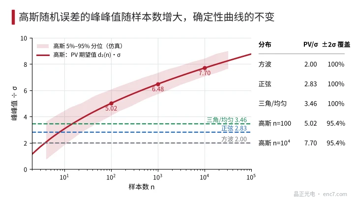
A mixed curve makes the point more clearly. A sine of amplitude 1 plus noise of σ = 0.1, at 3600 points per period: RMS rises only from 0.707 to 0.714 (+1%), but the mean peak-to-peak rises from 2.00 to about 2.57 (+28%). Peak-to-peak is set by a few points in the tails and is sensitive to noise and sample count; RMS is set by all points and is far more stable.
Combination: root-sum-square holds only for RMS-type quantities
When several mutually uncorrelated errors add, their variances add:
σ_tot² = Σσ_i² + 2·Σρ_ij·σ_i·σ_j
ρ_ij is the correlation coefficient; when the errors are uncorrelated the second term is zero, which is root-sum-square. Sines of different orders are orthogonal over a whole period, so for any phases the RMS obeys root-sum-square exactly. Peak-to-peak has no such property, and root-sum-square combination of peak-to-peak values comes out too small (for the statistics of combining harmonic peaks see the error-budget article in this library).
Worked example (illustrative): first harmonic of amplitude 10″ (PV 20″), interpolation error of a 2048-line disc of amplitude 2″ (PV 4″), noise σ = 0.5″, 65 536 samples per revolution.
| Combination method | Result |
|---|---|
| RMS root-sum-square √(7.07² + 1.41² + 0.5²) | 7.23″, matching the actual RMS of 7.23″ |
| PV root-sum-square √(20² + 4²) | 20.4″ |
| PV added directly | 24.0″ |
| Actual PV (with noise, simulated) | 26.9″ |
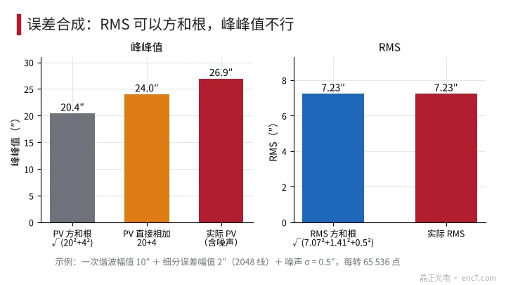
While the slowly varying first harmonic dwells near its crest, the fast interpolation error runs through dozens of periods, so there is always one period whose peak has the same sign; the peak-to-peak values of deterministic components should therefore be added directly, and noise added on top according to the sample count using d₂(n). The correct procedure is: convert each component to σ with its shape factor and find the total RMS by root-sum-square; when a peak-to-peak value is needed, convert back according to the actual shape of the combined curve or by simulation.
Misjudgements caused by mismatched bases
| Supplier reports | Customer understands | What is actually the case |
|---|---|---|
| RMS 3.5″ (mainly first harmonic) | ±3.5″ | ±4.95″, PV 9.9″ |
| 2σ = 5″ (mainly noise) | ±5″, PV 10″ | PV about 19.3″ on a 10 000-point record |
| Repeatability 2σ = 1″ (meaning full width of ±σ) | ±2σ = ±1″ | actual ±2σ is ±2″ |
| PV 5.0σ measured on 100 points | re-measured on 10 000 points PV 7.7σ, judged “worse” | the product is unchanged; the sample count changed |
| Individual PVs allocated by root-sum-square to 20.4″ | meets PV ≤ 22″ | measured PV about 26.9″, out of tolerance |
Engineering points
- A specification must state four things: the statistic (PV, ±PV/2, max|e|, RMS, σ), the zero (mean, midpoint or a particular line), the sample count and sampling range, and whether noise is included.
- Before comparing two data sets, convert them to the same quantity: PV ≈ 2.83σ when sine-dominated, about 3.46σ when triangle- or uniform-dominated, and by d₂(n) when noise-dominated.
- Always build error budgets by root-sum-square of σ or RMS; when an upper bound is needed, multiply by a coverage factor or simulate—never take root-sum-square of peak-to-peak values.
- For noise-dominated parameters, prefer to report σ and state the number of samples and the measurement bandwidth; when reporting peak-to-peak, also give the sample count, otherwise different measurement runs cannot be compared.
- When writing “2σ”, state that it is the half-width of ±2σ; only for approximately Gaussian error can it be said to cover about 95%—for a sine or a uniform distribution the ±2σ interval contains all samples.
Summary
Peak-to-peak looks at the extreme points, RMS and σ at the whole curve, and their ratio is set by the shape of the curve: 2 for a square wave, 2.83 for a sine, 3.46 for a triangle or uniform distribution, while for Gaussian random error it grows with sample count. Root-sum-square combination applies only to RMS-type quantities; before comparing specifications, convert the other party’s figure to your own basis.
Translated from the ENC7 Chinese technical library (article 0272). Read the Chinese original. Need a disc built to your drawing? Request a quote or see our custom encoder discs.
© Langfang Jingzheng Optoelectronic Technology Co., Ltd. All rights reserved. This article was created with AI assistance.