Custom discs
High Line Count at Small Radius or Low Line Count at Large Radius? Error Comparison at Equal Resolution
2²⁰ counts per revolution can be achieved with r = 10 mm and 4,096 lines interpolated 256×, or with r = 20 mm and 1,024 lines interpolated 1,024×. This article calculates eccentricity, interpolation, graduation, noise, gap and frequency item by item: with a single readhead the latter totals about 47″ and the former about 71″, and the critical eccentricity between the two schemes is about 0.6 μm.
To get 2²⁰ (1,048,576) counts per revolution, about 1.24″ per count, there are two routes: 4,096 lines at r = 10 mm interpolated 256×, or 1,024 lines at r = 20 mm interpolated 1,024×. Resolution is the same but the error makeup is completely different. The former has dense lines and a small radius — large eccentricity error and small interpolation error; the latter is the reverse. This article calculates the error components of both schemes and then says when to choose which.
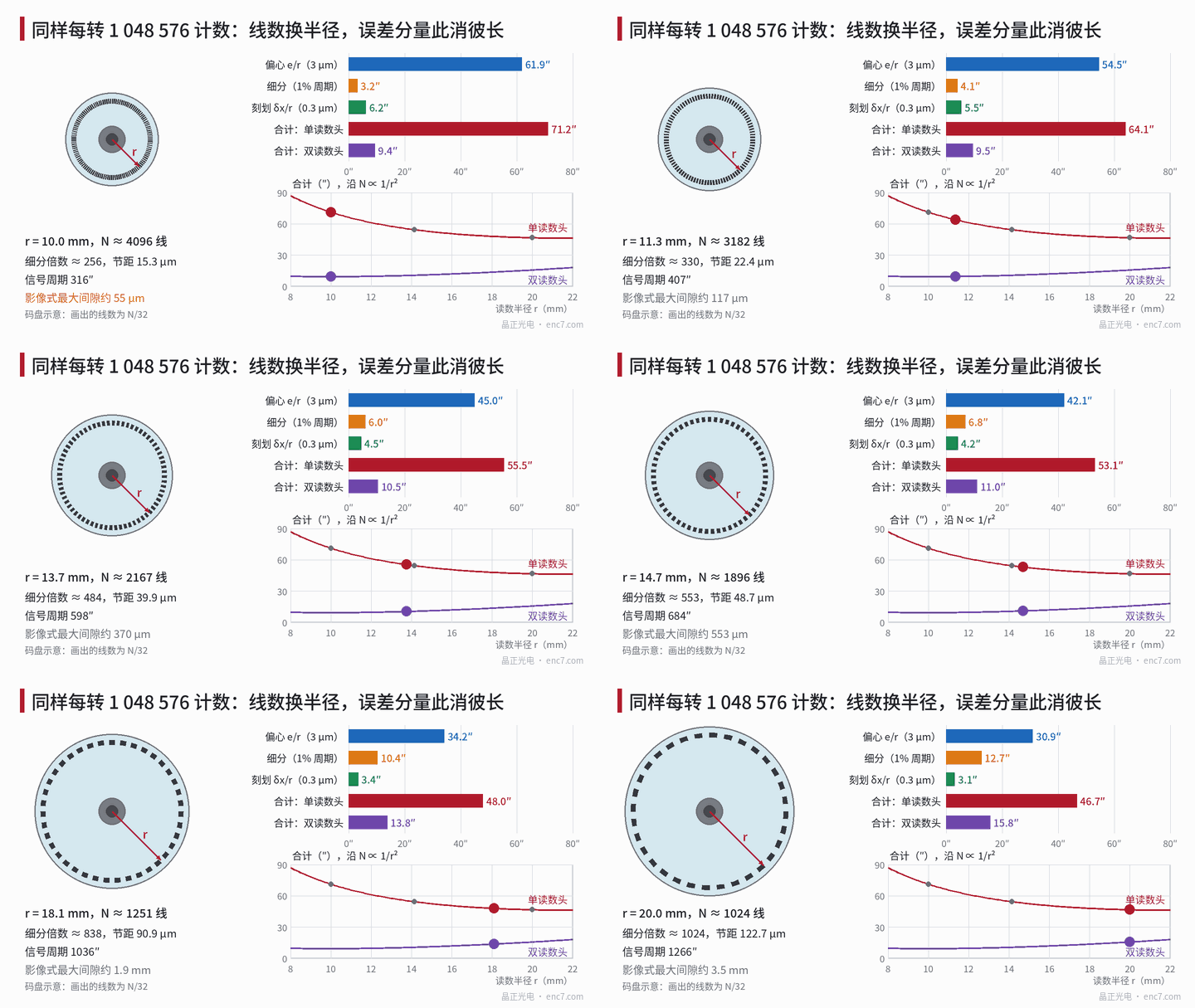
How each error component varies with r and N
Let read radius be r, line count N, interpolation factor k and counts per revolution C = N·k.
Eccentricity (single readhead, first harmonic): Δθ_e = e / r, where e is the offset of the pattern centre from the rotation axis.
Interpolation error: proportional to the signal period. Signal period P = 360°/N; if interpolation error is ε_i of a period (peak, a relative value set by signal quality), then Δθ_i = ε_i·P.
Graduation error: if it comes mainly from line position error δx (mask writing, exposure, substrate distortion), the angular error is Δθ_g = δx / r. If it comes from angular-type error (e.g. rotary-table error in polar writing), it is independent of r.
Noise: signal-relative noise σ_n/A converted to angle is σ_θ = (σ_n/A)·P/(2π), also proportional to period.
Gap: the maximum gap for imaging readout is about g_max ≈ 0.205·p²/λ (derivation in the library article on the line-count limit of imaging readout), with pitch p = 2πr/N.
Signal frequency: f = N·n/60, with n the speed (r/min).
So r enters only eccentricity, line-position-type graduation error and pitch; N enters only interpolation, noise, pitch and frequency. The difference between the schemes is the trade-off between these two groups.
Worked example: 10 mm/4,096 lines vs 20 mm/1,024 lines
Example assumptions: single-readhead residual eccentricity e = 3 μm, interpolation error 1% of period (uncompensated), δx = 0.3 μm, signal-to-noise A/σ_n = 500, λ = 0.88 μm.
| Item | A: r = 10 mm, 4,096 lines | B: r = 20 mm, 1,024 lines |
|---|---|---|
| Interpolation factor | 256 | 1,024 |
| Pitch | 15.3 μm | 122.7 μm |
| Signal period P | 316.4″ | 1,265.6″ |
| Eccentricity e/r | 61.9″ | 30.9″ |
| Interpolation error 1%·P | 3.2″ | 12.7″ |
| Graduation δx/r | 6.2″ | 3.1″ |
| Total (single readhead) | 71.2″ | 46.7″ |
| Total (two readheads, eccentricity cancelled) | 9.4″ | 15.8″ |
| Noise σ_θ | 0.10″ | 0.40″ |
| Maximum imaging gap | about 55 μm | about 3.5 mm |
| Signal frequency at 6,000 r/min | 409.6 kHz | 102.4 kHz |
| Disc OD (example) | about Φ24 | about Φ44 |
Totals are sums of component peaks. Eccentricity is a first harmonic, while interpolation error consists of harmonics at 1, 2 and 4 times per period; with orders differing by a factor of a thousand or more, the high-order terms run through many periods near the first-harmonic peak, so the peaks almost certainly coincide — adding peaks directly is not conservative.
The conclusion is clear: with one readhead, eccentricity accounts for 87% of scheme A, and scheme B halves it with double the radius, for a total about 24″ smaller; with two readheads cancelling eccentricity, what remains is mainly interpolation error, and scheme A’s period is only a quarter of B’s, so its total is about 6″ smaller instead.
Critical eccentricity: when the larger radius pays off
Setting the single-readhead totals equal, B beats A when
(e + δx)·(1/r_A − 1/r_B) > ε_i·(P_B − P_A)
with P in radians and r in mm. Substituting 1/r_A − 1/r_B = 0.05 mm⁻¹, P_B − P_A = 949.2″ ≈ 4.60 mrad and ε_i = 1% gives e + δx > 0.92 μm, i.e. a critical eccentricity e* ≈ 0.62 μm. With ε_i = 2%, e* ≈ 1.54 μm; with 0.5%, about 0.16 μm.
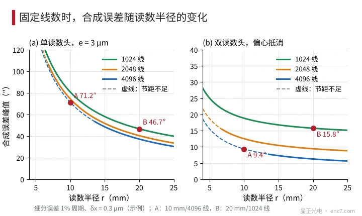
Residual eccentricity after assembly of a single-readhead encoder is generally on the micron scale, far above 0.6 μm, so low line count at large radius wins. Only with diametrically opposed dual readheads, on-shaft eccentricity compensation, or interpolation error that is already very small does the high line count’s advantage show. Figure 2 plots total error versus r for three line counts: at a given radius more lines is better, but 4,096 lines at 0.1 mm gap requires r ≥ 13.5 mm, and scheme A’s 10 mm falls on the dashed segment where pitch is insufficient.
Other costs
- Gap and readout method: scheme A’s 15.3 μm pitch requires an imaging gap below about 55 μm, leaving little margin for runout and axial play; it often needs interferential or three-grating readout instead. Scheme B’s gap is almost unconstrained.
- Signal frequency: scheme A is at 409.6 kHz at 6,000 r/min, and the front-end bandwidth and comparator must be designed for it; scheme B is a quarter of that.
- Interpolation circuit: scheme B divides each period into 1,024 parts, each about 6.1 mrad electrical, demanding more of noise and ADC resolution; its noise angle is 4× scheme A’s.
- Size and inertia: at the same thickness inertia grows with the fourth power of OD; Φ44 is about 11× Φ24. Usually minor for servo motors, but a hard constraint for space-limited joint modules.
Engineering notes
- First decide whether eccentricity can be cancelled: with one readhead it usually dominates combined error — about 87% for scheme A in the example — so increase read radius first.
- Use critical eccentricity to choose: e* = ε_i·(P_B − P_A)/(1/r_A − 1/r_B) − δx, about 0.6 μm in the example; if actual eccentricity exceeds it, choose low line count at large radius.
- With dual readheads or on-shaft compensation, look at interpolation error instead: it is proportional to signal period, and in the example the 4,096-line scheme totals 9.4″, better than the 1,024-line 15.8″.
- For high line count at small radius, check gap first: at r = 10 mm and 4,096 lines the pitch is 15.3 μm, and imaging gap must be below about 55 μm.
- For low line count at large radius, check the interpolation chain: noise angle is proportional to period, and the higher the interpolation factor, the higher the SNR required of ADC and analogue front end.
- Distinguish graduation error types: line-position type falls with larger r, angular type is independent of r; increasing radius only helps the former.
Summary
For the same resolution, the combination of line count and radius determines the error makeup: radius governs eccentricity and line-position error; line count governs interpolation error, noise and pitch. With a single readhead and micron-level eccentricity, low line count at large radius is more accurate; with eccentricity cancelled, high line count at small radius is more accurate, at the price of gap and bandwidth. Plug your own parameters into the critical-eccentricity formula to decide directly which route to take.
Translated from the ENC7 Chinese technical library (article 0302). Read the Chinese original. Need a disc built to your drawing? Request a quote or see our custom encoder discs.
© Langfang Jingzheng Optoelectronic Technology Co., Ltd. All rights reserved. This article was created with AI assistance.