Testing, reliability & quality
High-Speed Dynamic Testing: Encoder Error and Signal Integrity in Motion
An encoder that passes static calibration may, at 6000 r/min, show tens of arcseconds of position lag, interpolation error that grows with speed, and lost pulses. This article computes amplitude, phase and channel-mismatch effects with a first-order front-end model, gives the maximum-speed formula limited by edge spacing, and compares the reference-encoder method with the time-interval method.
A 2500-line encoder calibrated on a low-speed rotary table has less than 1″ of interpolation error. Mounted on a servo motor and run to 6000 r/min, the controller sees a position about 46″ behind reality, the shape of the error curve differs from the static one, and at the speed limit counts are occasionally lost. None of this is a graduation problem of the disc; these are dynamic errors that appear only “once it is turning”. This article discusses where they come from, how large they are, and how to measure them.
Static error versus dynamic error
Static error is measured at rest or at very low speed and includes graduation error, eccentricity and interpolation error from sine/cosine signal defects. It depends only on angular position, not on speed.
Dynamic error changes with speed and mainly comprises: amplitude drop and phase lag from limited signal-chain bandwidth; interpolation error from mismatched A/B frequency responses; lost pulses from the speed limits of counting, interpolation and receiving circuits; and mechanical factors such as shaft vibration and disc axial runout at high speed.
Speed and signal frequency are related by f = N·n/60, where N is the line count and n the speed (r/min). At 2500 lines and 6000 r/min, f = 250 kHz.
Analogue front end: amplitude, phase and channel mismatch
The photodiode junction capacitance and the transimpedance amplifier form a low-pass. Approximating with a first-order model:
|H| = 1 / √(1 + (f/f_c)²), φ = arctan(f/f_c)
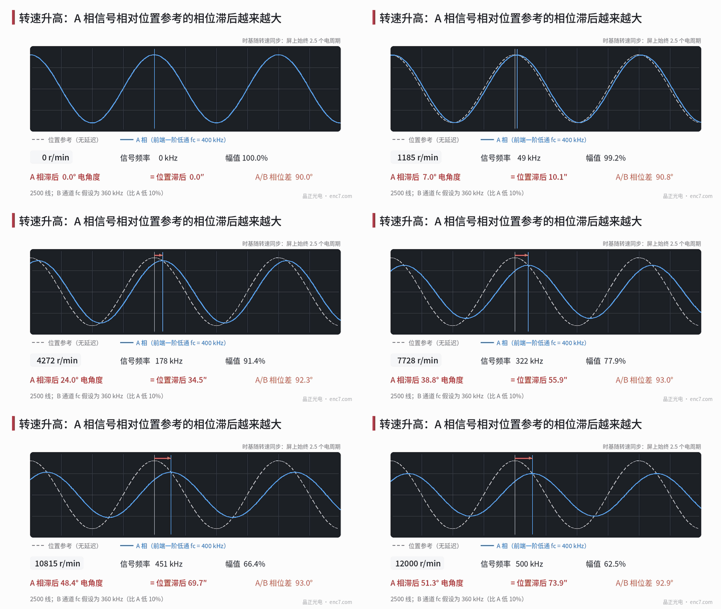
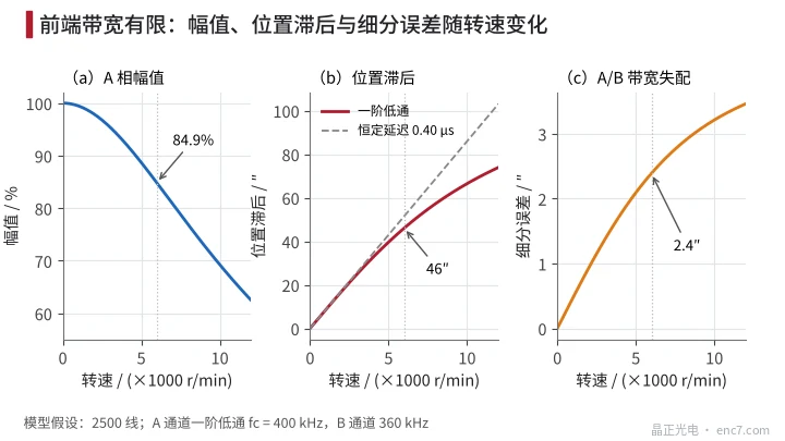
where f_c is the cut-off frequency and φ the phase lag. With f_c = 400 kHz (assumed), at 6000 r/min amplitude falls to 84.9% and phase lag is 32.0° electrical. Electrical angle divided by line count is mechanical angle: 32.0°/2500 = 0.0128°, i.e. about 46″ of position lag.
At low frequency a first-order low-pass is equivalent to a constant delay τ = 1/(2π·f_c) ≈ 0.40 μs, and the position lag Δθ = ω·τ is proportional to speed (Figure 2b). That lag is not a graduation error; when the delay is stable it can be compensated in the controller by speed; but if delay varies with temperature or device batch, compensation leaves a residual.
More subtle is channel mismatch. If channel B’s f_c is 10% lower than A’s (360 kHz), at 6000 r/min the phase difference between the two becomes about 92.8°, amplitudes differ by about 3%, and a 2-per-period interpolation error of about 2.4″ appears; at 12000 r/min it approaches 3.5″ (Figure 2c). Low-speed calibration never sees this term.
Digital path: edge spacing and lost pulses
For an encoder that outputs square waves after interpolation, counts per revolution are 4·N·k (k the interpolation factor). The counter or interpolation chip requires adjacent edges no closer than t_min, so the maximum speed is
n_max = 60 / (4·N·k·t_min)
At 2500 lines, ×25 interpolation and t_min = 100 ns, n_max = 2400 r/min. Real signals have phase error and jitter, so the minimum edge spacing is less than the average and margin is needed.
Cable also eats margin: a 5 ns skew between A and B differential pairs is only 0.45° electrical on a 250 kHz raw signal, but 5% of a 100 ns interpolated edge spacing.
An absolute serial encoder has no lost-pulse problem, but it has sampling delay. Delay τ corresponds to a position lag of 360°·(n/60)·τ; at τ = 1 μs and 6000 r/min that is about 0.036° (about 130″), and the controller must know exactly when position was sampled.
Dynamic amplification of small static errors
Position error is amplified when velocity is derived. For an error e·sin(kθ) with k cycles per revolution, the relative fluctuation of the velocity measurement is k·e. A 2-per-period interpolation error on a 2500-line encoder has k = 5000; at e = 1″ (4.85×10⁻⁶ rad) the velocity fluctuation is about 2.4%. At high speed that fluctuation frequency is far above the servo bandwidth and is filtered out; at low speed it falls inside the bandwidth as torque ripple and noise. So an encoder that is smooth at low speed needs small short-period error, not only high overall accuracy.
How to do dynamic testing
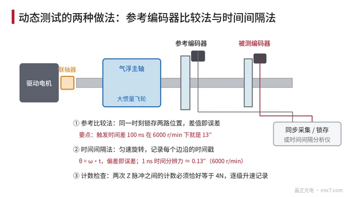
- Reference-encoder comparison: the encoder under test and a high-accuracy reference share an axis; at constant speed both positions are latched together and the difference is the error. Stepping the speed up and comparing with the low-speed curve separates the dynamic part. Synchronisation is critical: a 100 ns difference between the two latch instants is already a false error of 13″ at 6000 r/min; coupling torsion and shaft vibration must also be assessed separately.
- Time-interval method: a high-inertia air-bearing spindle runs at constant speed or coasts down; a time-interval analyser timestamps every edge; θ = ω·t converts time to angle and is compared with ideal equal division. No reference encoder is needed; at 6000 r/min a 1 ns time resolution corresponds to about 0.13″; the main error source is speed fluctuation within one revolution.
- Signal-integrity check: an oscilloscope watches amplitude versus speed, the high-speed Lissajous figure, and the differential-signal eye diagram with the actual cable length.
- Count check: the count between two successive Z pulses must equal exactly 4N (or 4·N·k for interpolated output); record while stepping speed up—any deviation means lost or extra counts.
Engineering points
- Accuracy in the specification should state the test speed; high-speed applications need a dynamic-error figure or the front-end bandwidth and delay.
- Front-end bandwidth should be well above the highest signal frequency (several times margin), and A/B channel device matching should be controlled; a 10% mismatch already produces about 2.4″ of high-speed interpolation error in this example.
- Position lag is proportional to speed and is a compensable term; what matters is delay stability—measure the temperature coefficient of delay when needed.
- For interpolated output check maximum speed with n_max = 60/(4·N·k·t_min) and leave margin for jitter and cable skew.
- Reference comparison must synchronise the two latches to the nanosecond; otherwise at high speed the false error far exceeds the error under test.
- Low-speed smoothness metrics should look at short-period error: 1″ of interpolation error at 2500 lines already corresponds to about 2.4% velocity fluctuation.
Summary
Encoder error splits into a static, angle-dependent part and a dynamic, speed-dependent part. Front-end bandwidth causes amplitude drop and a position lag proportional to speed; channel mismatch causes interpolation error that grows with speed; the digital path’s edge-spacing limit sets the highest speed without lost counts. Only reference comparison with synchronised latching, or the time-interval method, tested at several speeds, fully characterises an encoder in motion.
Translated from the ENC7 Chinese technical library (article 0198). Read the Chinese original. Need a disc built to your drawing? Request a quote or see our custom encoder discs.
© Langfang Jingzheng Optoelectronic Technology Co., Ltd. All rights reserved. This article was created with AI assistance.