Competing technologies and trends
Machine learning in encoder error compensation
Harmonic and look-up-table compensation are effective only for repeatable errors under the calibration conditions; the error changes when temperature or load changes. Using a set of illustrative data, this article compares static compensation, a physically structured model, a Gaussian process, a neural network and a high-order polynomial at interpolated and extrapolated temperatures, and sets out the points that matter for overfitting, cross-validation and interpretability.
Encoder error compensation is usually calibrated at one temperature and in one mounting condition, yielding a compensation table versus angle. Thermal mismatch between the hub and the shaft, however, changes the eccentricity, the readhead offset drifts with temperature, and load deforms the shafting, so the error in the field is not the same as the error at calibration. That has led to the suggestion of taking temperature, load and so on as inputs as well and fitting them with a machine-learning model. How far can this path be taken, and how does it relate to conventional harmonic compensation? This article uses a set of illustrative data to work out both the gains and the risks.
The error model: from e(θ) to e(θ, T, …)
Conventional compensation takes only the rotation angle θ as the independent variable:
e(θ) = Σ [a_k·cos(kθ) + b_k·sin(kθ)]
where k is the harmonic order per revolution and a_k, b_k are coefficients obtained by calibration. Once operating conditions are taken into account, the error becomes e(θ, x), where x may include temperature T, load, direction of rotation and so on. Common mechanisms include: thermal mismatch changing the eccentricity (mainly the 1st harmonic), load deforming the shafting (low-order harmonics), drift of the readhead offset (interpolation error 1 time per signal period), and reversal backlash (depending on the direction of rotation).
There are two modelling routes:
- Physically structured model: the harmonic form is kept and the coefficients are allowed to vary with operating conditions, for example a_k(T) = a_k0 + a_k1·(T − T₀). The model is linear in the parameters, so a single least-squares solution gives them all, and each coefficient has a physical meaning.
- Data-driven model: Gaussian-process regression, a small neural network, a gradient-boosted tree and the like, fitting the error directly with inputs such as cosθ, sinθ and T. Encoding θ as cosθ and sinθ is what makes the model satisfy 360° periodicity naturally.
Worked example: interpolation and extrapolation
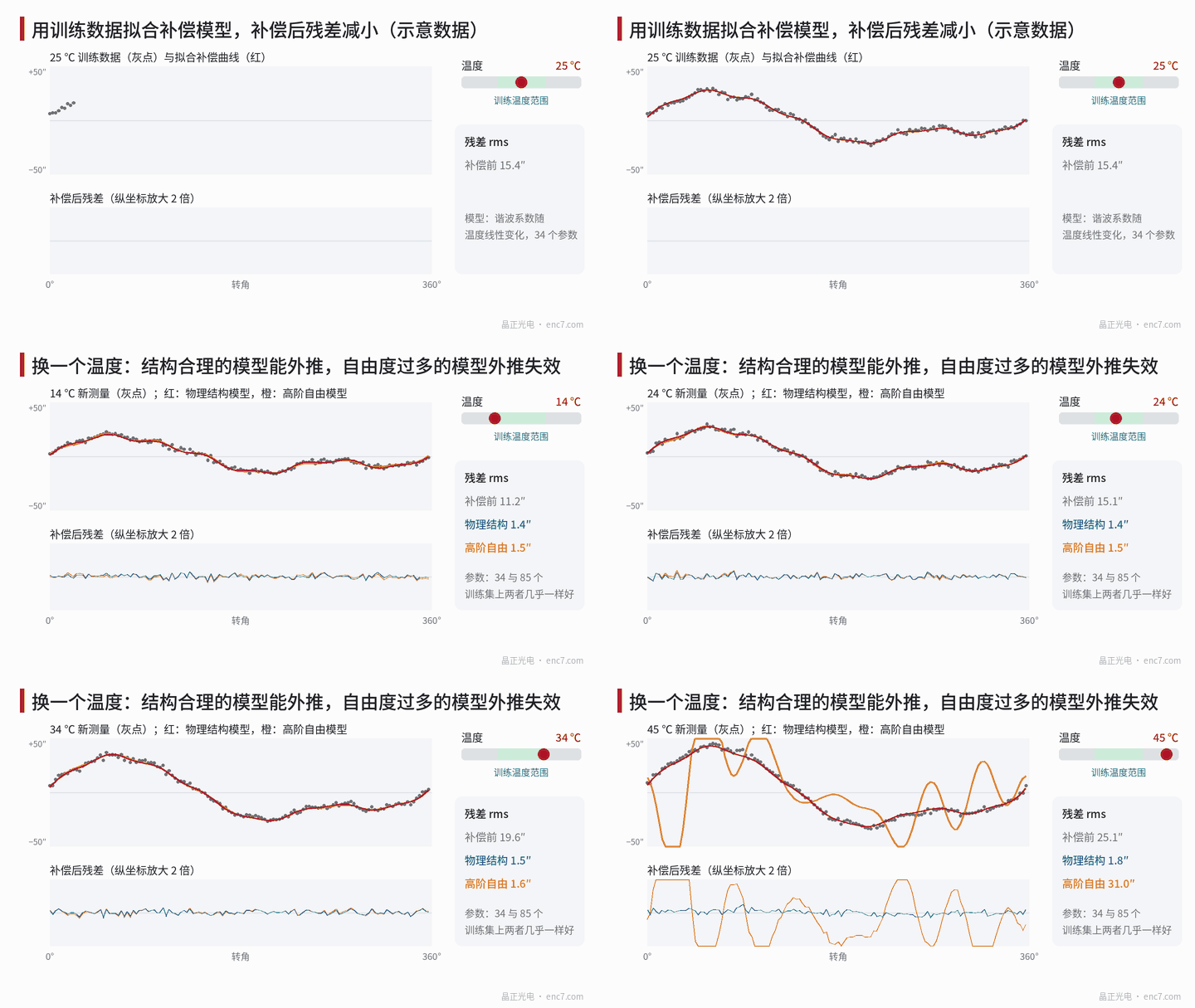
Illustrative data are constructed as follows: 1st-harmonic amplitude 20″ + 0.6″/K·ΔT + 0.004″/K²·ΔT², 2nd harmonic 8″ + 0.15″/K·ΔT, plus fixed 3rd-harmonic (3″) and 8th-harmonic (1.5″) components, measurement noise 1.5″ rms, and ΔT the temperature difference from 25 °C. At each of 15, 20, 25, 30 and 35 °C, 128 points are taken as training data, and test data are then acquired at new temperatures.
| Model | Number of parameters | 27.5 °C (interpolation) | 45 °C (extrapolation) | 5 °C (extrapolation) |
|---|---|---|---|---|
| Uncompensated | — | 16.7″ | 25.2″ | 8.2″ |
| Static compensation (25 °C only, 8th order) | 17 | 2.1″ | 10.1″ | 7.8″ |
| Physically structured (8th order, coefficients linear in T) | 34 | 1.5″ | 2.0″ | 1.9″ |
| Gaussian-process regression | Non-parametric, 640 points stored | 1.9″ | 1.9″ | 1.9″ |
| Neural network (2 layers × 32) | 1217 | 1.5″ | 4.8″ | 3.2″ |
| High-order unconstrained model (coefficients quartic in T) | 85 | 1.6″ | 31.2″ | 30.3″ |
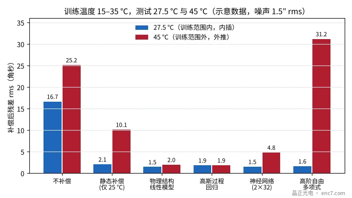
A few observations:
- Inside the training range, everyone looks much the same: except for static compensation, the residual of each model is close to the 1.5″ noise level. Looking only at interpolation performance, one cannot tell good models from bad.
- Extrapolation is where the difference appears: the physically structured model still has 2.0″ at 45 °C; the neural network degrades to 4.8″; the high-order unconstrained model reaches 31.2″, worse than the uncompensated 25.2″.
- The Gaussian process does well in this case, because it learned a long correlation length in the temperature direction from the data. Models of this kind, however, revert to the prior mean when far from the data, so extrapolation performance depends on the kernel and the hyperparameters and must not be taken as a general rule.
The conclusion from this data set is not that “machine learning does not work”, but that whether a model can extrapolate depends on whether its structure agrees with the physics, not on what it is called.
Overfitting and model selection
Training error falls monotonically with model complexity, so the model must be validated on data it has not seen. For temperature-dependent compensation, drawing test points at random is not reliable: points at the same temperature are highly correlated, and a random split will overstate the model’s performance. A more appropriate approach is leave-one-temperature-out cross-validation: each time, all the data at one temperature are held out, the remaining temperatures are used for training, and the held-out temperature is then predicted.
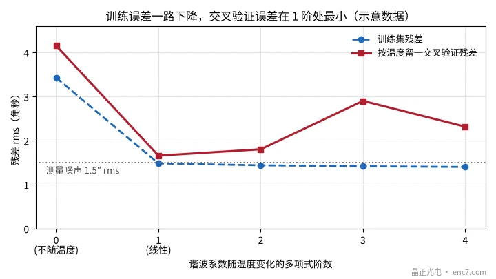
In the example, as the polynomial order goes from 0 to 4, the training residual falls from 3.43″ to 1.40″, already below the noise; the cross-validation residuals are 4.15″, 1.66″, 1.80″, 2.90″ and 2.32″ in turn, smallest at order 1. The number of parameters should also be set against the amount of data: 34 parameters for 640 points is comfortable, whereas a neural network with 1217 parameters relies mainly on regularization for constraint.
Interpretability, safety and deployment
- Interpretability: the coefficients of a physically structured model can be used directly for diagnosis — for example, the slope of the 1st harmonic with temperature corresponds to the eccentricity change caused by thermal mismatch, and an anomaly can be traced back to assembly or materials; the predictions of a black-box model are hard to check term by term.
- Define the domain of applicability: record the temperature and load ranges covered by the training, and alarm or fall back to a conservative compensation when operating conditions go outside them; at the same time limit the amplitude of the compensation so that the model cannot output an abnormal value.
- Functional safety: compensation changes the position value directly; when it is used in a safety-related function, the algorithm, the data and the tool chain must all be validated according to the procedures of standards such as IEC 61508.
- Computing load and latency: a physically structured model takes a few tens of multiply-adds per sample, a 2×32 neural network about a thousand multiply-adds; at update rates of several tens of kHz an embedded processor can generally carry the load, but latency and storage must be counted in.
- Drift and ageing: the model is based on the data of a given moment, so a re-inspection interval needs to be specified.
In the published literature, data-driven methods appear more often in research work and in machine-level thermal-error compensation; at the level of the encoder itself, harmonic and look-up-table compensation remain the mainstream. A more practical approach is a “grey box”: a physically structured model takes the main errors, a data-driven model fits the remainder, and the output of the latter is amplitude-limited.
Engineering points
- Compensate the repeatable error cleanly first: static harmonic compensation is still the foundation; in the example it reduces the error at an interpolated temperature from 16.7″ to 2.1″.
- Write the physical structure into the model: a model whose coefficients vary linearly with temperature has only 34 parameters and is stable in both interpolation and extrapolation.
- Validate leave-one-condition-out: hold out whole groups by temperature or by load; do not draw points at random, or the effect will be overstated.
- Training coverage must be wider than the range of use: in the example the high-order unconstrained model is worse than no compensation when extrapolating to 45 °C.
- Encode the periodicity in the inputs: use cosθ and sinθ as inputs, not θ itself.
- Limit the amplitude in deployment and monitor the domain of applicability: alarm or fall back to a conservative compensation when the training range is exceeded.
Summary
Machine learning can bring operating conditions such as temperature and load into error compensation, but inside the training range it differs little from a physically structured model; the differences appear in extrapolation, interpretability and the cost of validation. What decides success or failure is the model structure, the data coverage and the validation method. For encoders, a harmonic physical model as the backbone, with a data-driven model as a supplement, is at present the more robust route.
Translated from the ENC7 Chinese technical library (article 0188). Read the Chinese original. Need a disc built to your drawing? Request a quote or see our custom encoder discs.
© Langfang Jingzheng Optoelectronic Technology Co., Ltd. All rights reserved. This article was created with AI assistance.