Testing, reliability & quality
SPC Control Charts in Encoder-Disc Production
Staying inside tolerance does not mean the process is stable. Using encoder-disc line width as an example, this article fully calculates X̄-R control limits from simulated data (A₂, D₃, D₄ constants), explains run rules, rational subgroups and ARL, and distinguishes control limits from tolerance limits.
Encoder-disc line width is specified at 25.0 ±1.0 μm, and every inspection record over the past three months has been conforming. One day, after a developer change, line width starts to creep wider—only a few hundredths of a micrometre per batch, still far from the upper tolerance, so inspection keeps passing everything. By the time a nonconforming piece appears, dozens of batches may already be running off-centre. What statistical process control (SPC) must do is detect that the process has changed while product is still conforming.
The X̄-R chart and control limits
Each time, n pieces are drawn from continuous production to form a subgroup; the subgroup mean X̄ and range R are computed. After accumulating k subgroups (generally at least 20–25), the grand average of the subgroup means CL (centre line) and the average range R̄ are obtained; the control limits are:
UCL_X = CL + A₂·R̄, LCL_X = CL − A₂·R̄ UCL_R = D₄·R̄, LCL_R = D₃·R̄
The constants come from the statistical properties of the range under a normal distribution. Writing d₂ for the ratio of the expectation of R to σ and d₃ for the ratio of the standard deviation of R to σ, then A₂ = 3/(d₂·√n), D₄ = 1 + 3d₃/d₂, D₃ = max(0, 1 − 3d₃/d₂). For n = 5, d₂ = 2.326 and d₃ = 0.864, so:
| Subgroup size n | A₂ | D₃ | D₄ | d₂ |
|---|---|---|---|---|
| 4 | 0.729 | 0 | 2.282 | 2.059 |
| 5 | 0.577 | 0 | 2.114 | 2.326 |
The process standard deviation is estimated as σ̂ = R̄/d₂.
Line-width worked example
Simulated data: 5 discs per subgroup, Phase I with 25 subgroups (assumed process mean 25.05 μm, standard deviation 0.15 μm). Calculation gives:
- CL = 25.056 μm, R̄ = 0.357 μm
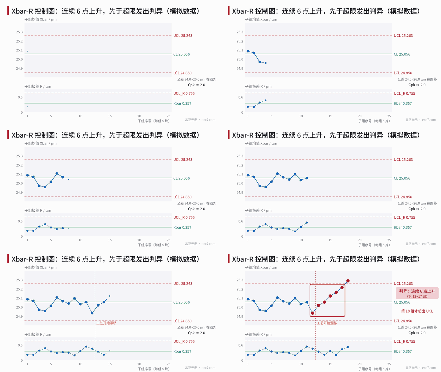
- UCL_X = 25.056 + 0.577 × 0.357 ≈ 25.263 μm, LCL_X ≈ 24.850 μm
- UCL_R = 2.114 × 0.357 ≈ 0.755 μm, LCL_R = 0
- σ̂ = 0.357 / 2.326 ≈ 0.154 μm, Cp ≈ 2.17, Cpk ≈ 2.05
All Phase I points lie inside the control limits with no abnormal patterns, so the limits can be used for Phase II monitoring. In Phase II, from subgroup 13 the mean drifts +0.03 μm per subgroup (simulating a development-condition change). At subgroup 17, subgroups 12–17 show 6 consecutive rising points and trigger a run rule; by then the mean has shifted only about 0.15 μm and every individual value is still inside tolerance. Only subgroup 18 exceeds the upper control limit.
It should be noted that this data set was constructed for demonstration. For a linear drift, which of “consecutive rise” or “out of control limits” fires first depends on the ratio of drift rate to the random variation of the subgroup mean; the trend rule is not always first.
Run rules and false alarms
The commonly used run rules (Nelson rules) are 8: 1 point beyond the 3σ control limits; 9 consecutive points on the same side of the centre line; 6 consecutive points increasing or decreasing; 14 consecutive points alternating up and down; 2 of 3 points beyond 2σ on the same side; 4 of 5 points beyond 1σ on the same side; 15 consecutive points inside ±1σ; 8 consecutive points outside ±1σ. The later rules correspond respectively to drift, periodicity, stratification and mixture process states.
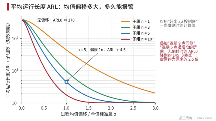
More rules are not always better. When the process has not changed, using only rule 1 gives on average one false alarm every 370 subgroups (ARL₀ ≈ 370); after adding “9 points same side” and “6 points increasing/decreasing”, Monte Carlo simulation gives ARL₀ about 145, so the false-alarm frequency is about 2.5 times the original.
Detection power is measured by the average run length (ARL) (Figure 3). For a mean shift of 1 individual-value standard deviation, an X̄ chart with n = 5 alarms after 4.5 subgroups on average; with n = 1 (individuals chart) it takes 44 subgroups on average.
Control limits are not tolerance limits
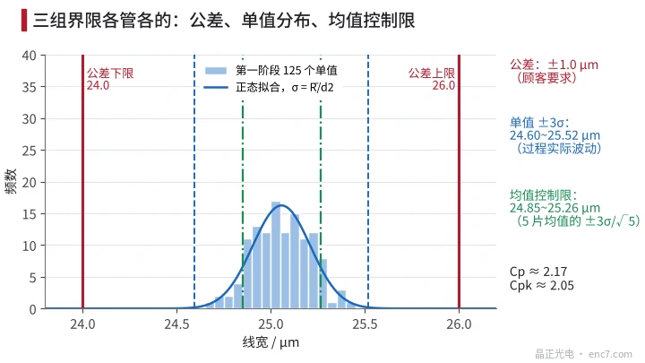
These three sets of limits are often confused (Figure 2):
- Tolerance limits (24.0–26.0 μm) are the customer’s requirement, used to decide whether a single piece conforms;
- Individual ±3σ (about 24.60–25.52 μm) is the process’s own variation range; comparing it with the tolerance yields process capability;
- Mean control limits (24.85–25.26 μm) are the variation range of the subgroup mean, used only to judge whether the process is stable.
Do not draw tolerance limits on the X̄ chart, and do not “widen” control limits with the tolerance. A process in control is not the same as adequate capability, and adequate capability is not the same as a process in control: in this example Cpk is about 2.05, yet the drift must still raise an alarm because it shows a special cause is acting.
Rational subgroups and the measurement system
How subgroups are taken decides what the control chart is monitoring. If the 5 values come from 5 positions on the same disc, R reflects only within-disc variation, control limits become too narrow, and normal batch-to-batch differences will frequently trigger run rules. For a parameter such as line width that varies by batch (same exposure and development), several discs from the same batch are often taken as a subgroup; when between-batch variation is large, an individuals–moving-range chart can be used on batch means together with a within-disc range chart.
Also, what the control chart sees is “process variation + measurement variation”. If the standard uncertainty of the line-width measurement is 0.09 μm, it accounts for about one third of the variance in the total standard deviation of 0.154 μm. Before running SPC, the measurement system should be assessed first.
Engineering points
- In Phase I accumulate at least 20–25 subgroups, recalculate control limits after removing points whose special causes have been identified, then move to monitoring.
- Look up control-chart constants by subgroup size: for n = 5, A₂ = 0.577, D₃ = 0, D₄ = 2.114, d₂ = 2.326.
- Match subgroups to the source of variation: organise subgroups by batch; avoid using only multiple points within one disc, or control limits will be too narrow and false alarms frequent.
- Choose run rules as needed; each added rule raises false alarms; in this example adding two trend-type rules raises false alarms about 2.5×.
- Tolerance limits are only for conformity decisions and are not drawn on the mean chart; a process with high Cpk still needs a response when a special-cause alarm fires.
- Process-condition changes (developer change, light-source change, mask change) should be annotated on the chart; recalculate Phase I when necessary.
Summary
The X̄-R control chart converts the average range of subgroup data into control limits with A₂, D₃ and D₄, and uses run rules to identify special causes in the process. It and tolerance decisions answer two different questions: the former asks “has the process changed?”, the latter “is the product conforming?”. With rational grouping, appropriate rules and a confirmed measurement system, the chart can detect process drift early while product is still conforming.
Translated from the ENC7 Chinese technical library (article 0200). Read the Chinese original. Need a disc built to your drawing? Request a quote or see our custom encoder discs.
© Langfang Jingzheng Optoelectronic Technology Co., Ltd. All rights reserved. This article was created with AI assistance.