Troubleshooting: Lissajous Centre Walks with Angle — Once-per-Revolution Offset Drift

When the Lissajous centre walks within one revolution, static correction is ineffective and auto-calibration still leaves residual. This article derives the angle-updated auto-cal residual ratio x/√(1 + x²), x = 2π·k·M_p/N: smooth walk can be cut by about nine-tenths, while a few-degree-wide local haze patch is left almost intact; it also gives locating by Z-segmented centre fitting and uniformity-metric recommendations.

The previous article treated offset as a constant that one correction removes. A harder case: turn the disc slowly and the Lissajous centre moves with angle, returning after one revolution. Offset then varies with angle; factory static correction is valid only at one angle, and online auto-calibration must “chase” it — what it cannot catch becomes residual. This article answers three questions: why offset varies with angle; how to measure the trajectory and locate it on the disc; how fast auto-cal can chase, and what uniformity metrics the disc should carry.

Figure 1 – Over one disc revolution, the Lissajous centre is computed once per signal period and joined into a closed trajectory in the A–B plane: a smooth small loop from slow non-uniformity; a large polygonal loop from a local haze patch sweeping the four sector detection fields (example model).

Why offset varies with angle

Offset comes from unequal DC seen by the 0° and 180° channels. The two detection fields look at different disc locations, so any circumferential non-uniformity of the disc becomes angle-dependent offset. With tangential field spacing d and clear-area transmittance varying slowly along arc length s:

ε(φ) ≈ −(d/(2M)) · (1/D)·dD/ds

where M is modulation and D is DC. For transmittance undulating u, k times per revolution, offset amplitude is about d·u·k/(2M·r).

Two worked examples (assumed): d = 1 mm, r = 20 mm, M = 0.5, slow 5% transmittance variation per revolution → ε only about 0.25%; a local haze patch covering one sector field with 5% lower transmittance → about 5% offset. Slow non-uniformity has limited effect; local abrupt change is the main issue.

Common sources:

Film or OD non-uniformity: chrome leakage or residual film in clear areas varying around the circumference.
Local haze: wash residue, adhesive mist, fingerprint marks — local transmittance drop with scatter.
Reflective-disc background: reflectance or surface state of non-reflecting areas inconsistent around the circle; with disc tilt the reflected spot also swings once per revolution.
Hub-edge reflections: screw heads, notches or steps on hub or clamp ring rotate with the disc and at some angles reflect light into one channel.

Phase-interleaved arrays in one window, with phases less than one period apart, are insensitive to this class of non-uniformity; sector detection-field structures are far more sensitive.

Locating: Z-segmented centre fit and trajectory

Acquire: fixed low constant speed, DC coupling, sample A, B and Z together; at least 20 points per signal period, continuously for one revolution or more.
Segment: unwrap phase from atan2; cut a segment each time phase increases by 2π — one signal period per segment — with Z as mechanical-angle zero.
Find the centre: average A and B inside each segment. Full-period average is unaffected by harmonics, amplitude difference and phase error and is that period’s centre; when noisy, least-squares circle-fit every K periods and Z-synchronously average multiple revolutions.
Plot: draw the (ε_A, ε_B) trajectory in the A–B plane and ε_A, ε_B versus angle.

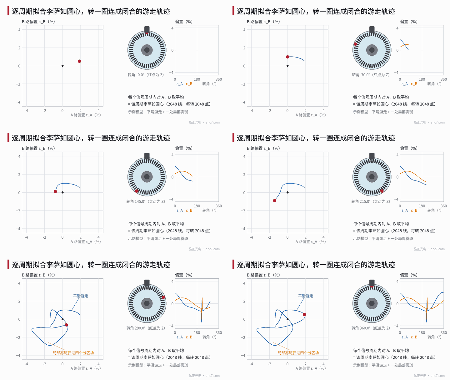
Reading the plot: a smooth closed small loop, 1–2 times per revolution, points to slow film/OD/reflection-background variation or hub-eccentricity-driven reflection change; a polygonal loop that suddenly shoots out at a fixed angle points to local haze or a hub feature — under sector fields a haze patch sweeps A+, B+, A−, B− in turn and bias shifts toward −A, −B, +A, +B forming a small square loop (Figure 1). Centre that does not move with angle but sits offset is a readhead-side problem. Once the angle is known, verify that clear area under a microscope or dark-field illumination with Z as reference.

Offset rate of change and auto-cal time constant

Suppose auto-cal updates once per signal period with memory of about M_p periods:

ε̂_m = ε̂_(m−1) + (ε_m − ε̂_(m−1)) / M_p

For slow change it acts as a low-pass filter; residual ≈ memory length × offset change per period. For offset varying k times per revolution let

x = 2π·k·M_p / N

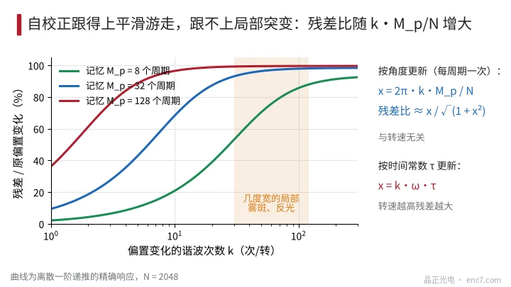
Residual-to-original ratio ≈ x/√(1 + x²), N = line count. Exact discrete recurrence at 2,048 lines:

Memory M_p	k = 1	k = 2	k = 8	k = 64
8 periods	2.1%	4.3%	17%	77%
32 periods	9.5%	19%	60%	97%
128 periods	36%	61%	95%	99.5%

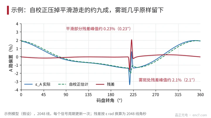
A few-degree-wide local haze patch is equivalent to tens of cycles per revolution; no reasonable memory length can catch it (Figure 2). In the Figure 3 example, at M_p = 32 the smooth-walk residual peak is about 0.23% (≈ 0.23″ at 2,048 lines) while the haze residual is about 2.1% — left almost intact.

With angle update, x is independent of speed; if auto-cal uses a fixed time constant τ, x = k·ω·τ grows with speed: at τ = 1 ms, k = 1, residual ≈ 3% at 300 r/min and ≈ 30% at 3,000 r/min. Error that is “good at low speed, bad at high” should first be checked for the auto-cal update mode. M_p cannot be shortened without limit: coverage below one period makes ellipse fitting ill-conditioned, and too-short memory “corrects” noise and harmonic error as if they were offset.

Figure 2 – Angle-updated auto-cal residual ratio for offset varying k times per revolution: smooth walk can be tracked; a few-degree local jump (orange region) essentially cannot.

Figure 3 – Example: A-channel offset over one revolution, auto-cal estimate (M_p = 32) and residual; smooth part ≈ 0.23%, haze ≈ 2.1% (example model).

Uniformity-metric recommendations

Let ε_r be the residual offset budget allocated in the previous article, and M_p the auto-cal memory; then disc- and assembly-driven offset variation should satisfy (example approach):

Slow part: amplitude ε_k of k×/rev offset ≤ ε_r·√(1 + x²)/x; for small x ≈ ε_r·N/(2π·k·M_p). At 2,048 lines, M_p = 32, ε_r = 0.5%: about 5.1% allowed at k = 1, 2.6% at k = 2 — generally easy.
Local jump: auto-cal essentially useless; local offset bump is capped directly at ε_r. With sector fields, M = 0.5, ε_r = 0.5%, local transmittance difference within one detection field must stay under about 2M·ε_r = 0.5% — haze invisible to the eye can already fail.
Disc inspection: clear-area transmittance along the track checked at two scales — millimetre-scale local undulation and full-circle slow variation, each with its limit; phase-interleaved readheads can relax the local limit.
Assembly: blacken or make non-reflecting hub and clamp-ring surfaces near the read zone; keep screw heads and notches away from the read zone.

Engineering notes

Centre walking with angle means offset is a function of position; static correction fails — measure the trajectory before talking about correction.
Averaging A and B over each signal period yields the centre; Z-segmenting and multi-revolution synchronous averaging draw a reliable trajectory.
Smooth small loop → slow film/OD/reflection background; fixed-angle polygonal loop → local haze and hub features.
Angle-updated auto-cal residual ratio ≈ x/√(1 + x²), x = 2π·k·M_p/N, independent of speed; time-updated residual rises with speed.
Local jumps cannot be chased — only disc cleanliness and transmittance uniformity solve them; sector-field readheads are stricter.
Incoming disc inspection should add local clear-area transmittance uniformity, with limits tiered by readhead architecture.

Summary

Offset walking with angle means the two detection fields see non-uniform disc regions. Z-segmented centre trajectories separate slow non-uniformity from local haze and locate them to a specific angle. Auto-cal works on the slow part with residual ratio ≈ x/√(1 + x²), and is essentially useless on a few-degree local jump, so uniformity metrics must split slow and local scales.

Translated from the ENC7 Chinese technical library (article 0208). Read the Chinese original. Need a disc built to your drawing? Request a quote or see our custom encoder discs.