Troubleshooting
Troubleshooting: Lissajous Turns from a Circle into a Tilted Ellipse at Higher Speed — Mismatched Channel Bandwidths
A Lissajous figure that is a circle at low speed but becomes a tilted ellipse as speed rises usually means channels A and B have different bandwidths: with 500 and 450 kHz the phase difference at 200 kHz is about 2.2°. This article derives how phase difference and amplitude ratio vary with frequency, shows how to distinguish channel delay from sampling skew, and gives measurement by speed steps and by light-modulation sweep at standstill, together with the bandwidth-matching tolerance.
During low-speed calibration on the test bench everything is fine and the Lissajous figure is a textbook circle; mounted on the motor and run at five to six thousand r/min, the same readhead’s Lissajous becomes a tilted ellipse, interpolation error grows with it, and everything recovers once the motor stops. This kind of phase error that “only appears at high speed” is most often caused by different bandwidths in the analogue A and B channels. This article derives how it varies with frequency, explains how to distinguish it from channel delay and sampling skew, how to measure it, and how closely the two bandwidths must be matched. How the bandwidth itself is set by photodiode capacitance and transimpedance is covered in the library article on photodiode capacitance and bandwidth.
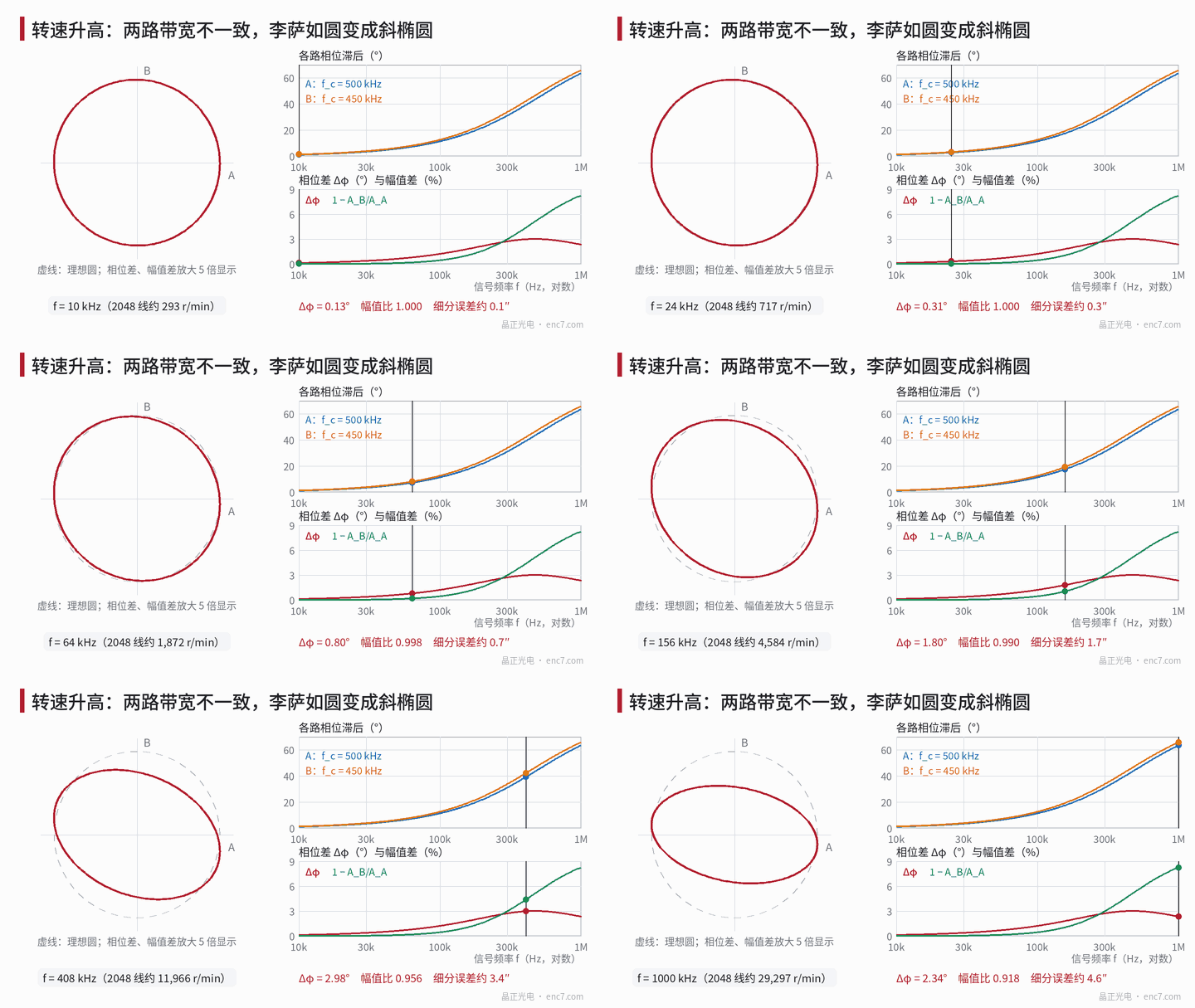
Model: phase difference and amplitude ratio versus frequency
Approximate each channel’s front end as a first-order low-pass H = 1/(1 + j·f/f_c), with cut-off frequencies f_A and f_B for channels A and B. The difference in phase lag and the amplitude ratio of the two channels are
Δφ = arctan(f/f_B) − arctan(f/f_A)
ρ = A_B/A_A = √(1 + (f/f_A)²) / √(1 + (f/f_B)²)
where f = N·n/60 is the signal frequency, N the line count and n the rotational speed (r/min). With f_A = 500 kHz, f_B = 450 kHz and f = 200 kHz, the lags are 21.80° and 23.96°, a difference of 2.16°; the amplitude ratio is 0.984.
These formulas have three properties worth remembering:
- At low frequency it looks like a fixed delay. For f well below the cut-off frequencies, Δφ ≈ 360°·f·Δτ with Δτ = (1/f_B − 1/f_A)/(2π) — 35 ns in the example.
- The phase difference has a peak. It is largest at f = √(f_A·f_B) ≈ 474 kHz, Δφ_max = arctan[(f_A − f_B)/(2√(f_A·f_B))] ≈ 3.0°, and decreases beyond that.
- The amplitude difference increases monotonically. It grows as f² at low frequency and tends to 1 − f_B/f_A = 10% at high frequency.
The phase difference tilts the ellipse along 45°, the amplitude difference flattens it along the axes; both produce an interpolation error twice per period with amplitude about ½·√(Δφ² + δ²) (δ = 1 − ρ, both in radians). In addition there is a fixed offset of Δφ/2, seen as a speed-dependent position lag. Converted for 2048 lines (1 rad electrical ≈ 100.7″):
| f | Speed at 2048 lines | Δφ | Amplitude difference δ | Interpolation error |
|---|---|---|---|---|
| 50 kHz | 1465 r/min | 0.63° | 0.1% | 0.56″ |
| 100 kHz | 2930 r/min | 1.22° | 0.5% | 1.09″ |
| 200 kHz | 5859 r/min | 2.16° | 1.6% | 2.06″ |
| 300 kHz | 8789 r/min | 2.73° | 3.0% | 2.82″ |
In the first three rows the error is almost proportional to frequency — the origin of “the faster, the worse”. A direct atan2 simulation gives an error amplitude of 0.0205 rad at 200 kHz, consistent with the approximation.
Distinguishing it from other speed-dependent causes
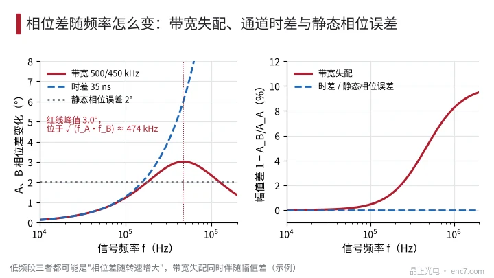
Speed-dependent phase error has more than one source, and each has its own frequency behaviour (see Figure 2):
| Cause | Δφ vs f | Amplitude ratio vs f | Analogue Lissajous on the oscilloscope |
|---|---|---|---|
| Mismatched channel bandwidths | Grows linearly at first, peaks at √(f_A·f_B), then falls | Decreases, starting as f² | Tilted and flattened ellipse |
| Channel delay Δt (filter group delay, comparator, traces) | 360°·f·Δt, keeps growing linearly | Unchanged | Tilted ellipse |
| Static phase error (readhead azimuth, detection-field layout) | Independent of speed | Unchanged | Already a tilted ellipse at low speed |
| Time-multiplexed A/B sampling on the digital side | 360°·f·Δt_s | Unchanged | Still a circle |
The last item is easily overlooked: when one ADC samples A and B alternately, the sampling interval Δt_s creates a phase difference in the digital domain; the analogue signals look perfectly normal on the oscilloscope, yet the interpolation error grows linearly with speed. So the first step is to check whether the “analogue Lissajous” and the “digital interpolation error” agree.
Measurement: speed steps and light-modulation sweep at standstill
Lissajous at stepped speeds. Choose 6–8 speeds across the maximum speed range; at each, capture A and B simultaneously with differential probes, fit an ellipse to get Δφ and ρ, plot against f = N·n/60, and fit Δφ = φ₀ + 360°·f·Δt + [arctan(f/f_B) − arctan(f/f_A)] — this separates the three components. Calibrate the skew of the oscilloscope channels and probes first: measure once with the probes swapped and average to cancel it.
Light-modulation sweep at standstill. If high-speed running is impractical, stop the shaft near 45°, where A and B have equal amplitude, open the constant-light loop, superimpose a small sinusoidal modulation (5%–10% depth) on the LED current from a signal generator, sweep from 10 kHz to 1 MHz and measure the ratio of the AC components at the A and B outputs. Because both channels see the same intensity modulation, the ratio is H_B/H_A, and the LED’s own bandwidth cancels in the ratio. Channel offsets add an extra term to the AC components; measuring once at 45° and once at 225° and taking the difference removes it. The upper limit of this method is set by the modulation bandwidth and signal-to-noise ratio of the LED drive.
If the circuit board is accessible, a test current can also be injected through a small capacitor into each transimpedance input to measure each channel’s transfer function directly.
Bandwidth-matching tolerance
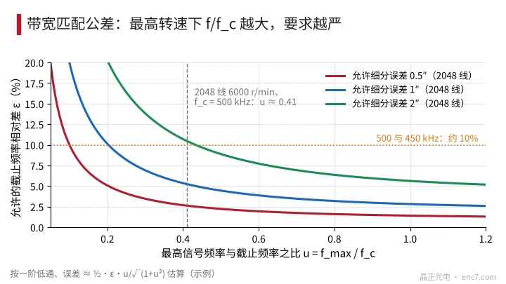
Let the relative difference of the cut-off frequencies be ε = (f_A − f_B)/f_A and the ratio of maximum signal frequency to cut-off frequency u = f_max/f_c. For small ε the error is about ½·ε·u/√(1 + u²), so for a given allowed error E (electrical angle, rad):
ε ≤ 2E·√(1 + u²) / u
Allowed values for 2048 lines:
| Allowed error | u = 0.2 | u = 0.4 | u = 0.8 |
|---|---|---|---|
| 0.5″ | 5.1% | 2.7% | 1.6% |
| 1″ | 10.1% | 5.3% | 3.2% |
| 2″ | 20.3% | 10.7% | 6.4% |
Example: 2048 lines at 6000 r/min gives f_max ≈ 205 kHz; with f_c = 500 kHz, u ≈ 0.41. For a high-speed interpolation error of no more than 1″, the difference between the two cut-off frequencies must be held within about 5% (see Figure 3).
Where the mismatch comes from: with 1% filter resistors and 5% capacitors the RC product can differ by about 6% in the worst case; transimpedance bandwidth is roughly inversely proportional to the square root of input capacitance, so a 10% difference in photodiode or trace capacitance between channels gives about 5% bandwidth difference; spread in op-amp gain-bandwidth product also enters as a square root. Countermeasures: use capacitors of 1%–2% from the same batch and one dual op-amp for both channels, with a symmetrical layout; if necessary raise f_c to lower u, while checking the extra noise this brings.
Engineering notes
- First convert speed into signal frequency with f = N·n/60, then look at the curves of Δφ and amplitude ratio versus f, rather than at one speed only.
- At low frequency a bandwidth mismatch is equivalent to a delay of Δτ = (1/f_B − 1/f_A)/(2π); for 500/450 kHz about 35 ns.
- How to tell: bandwidth mismatch brings an amplitude difference as well, and its phase difference peaks; a delay gives a purely linear phase; static error is present even at low speed; sampling skew is invisible on the analogue Lissajous.
- When high-speed running is impractical, measure H_B/H_A by light-modulation sweep at standstill, once at 45° and once at 225° to cancel offsets.
- Set the bandwidth-matching tolerance by ε ≤ 2E·√(1 + u²)/u — about 5% for 2048 lines, u = 0.4 and 1″; choose 1%–2% capacitors from the same batch and in the same package.
Summary
When the Lissajous figure becomes a tilted ellipse as speed rises, the two channels’ low-pass bandwidths usually differ: the phase difference first grows linearly with frequency and peaks at √(f_A·f_B), while the amplitude difference keeps increasing, and over the usual speed range the error is roughly proportional to speed. Separate it from delay, static error and sampling skew by fitting over speed steps or by light-modulation sweep at standstill, then derive the bandwidth-matching tolerance from the allowed error — that keeps it under control both in design and at incoming inspection.
Translated from the ENC7 Chinese technical library (article 0223). Read the Chinese original. Need a disc built to your drawing? Request a quote or see our custom encoder discs.
© Langfang Jingzheng Optoelectronic Technology Co., Ltd. All rights reserved. This article was created with AI assistance.