Troubleshooting
Troubleshooting: Sine Signal Tops Clipped Flat — Small Gap, Saturation or Squaring?
Clipped tops come in two kinds. Circuit saturation flattens the signal at a fixed level, independent of gap. Optical squaring happens at small gaps, where the signal approaches the convolution of the disc’s square wave with the detector element, and the 3rd and 5th harmonics grow. This article gives the harmonics and interpolation error of each, comparison tests by reducing gain and adjusting gap, and a method to estimate error from the flat-top fraction.
On the oscilloscope the A-phase sine is flat at both top and bottom. The line explanation is often “the gap is too small, the signal has become a square wave”, but the same flat top can also be amplifier or ADC saturation. Both look nearly square on the Lissajous figure, yet their effect on interpolation error differs and the remedies are entirely different: one needs lower gain, the other a gap adjustment or a different detector element. This article puts the models, signatures and comparison tests of both kinds of clipping side by side, and gives a way to estimate interpolation error from the degree of clipping. The general pattern of the 3rd harmonic oscillating with gap is covered in the “squircle” article in this series; here only the flat-top symptom is discussed.
Signatures of the two kinds of clipping
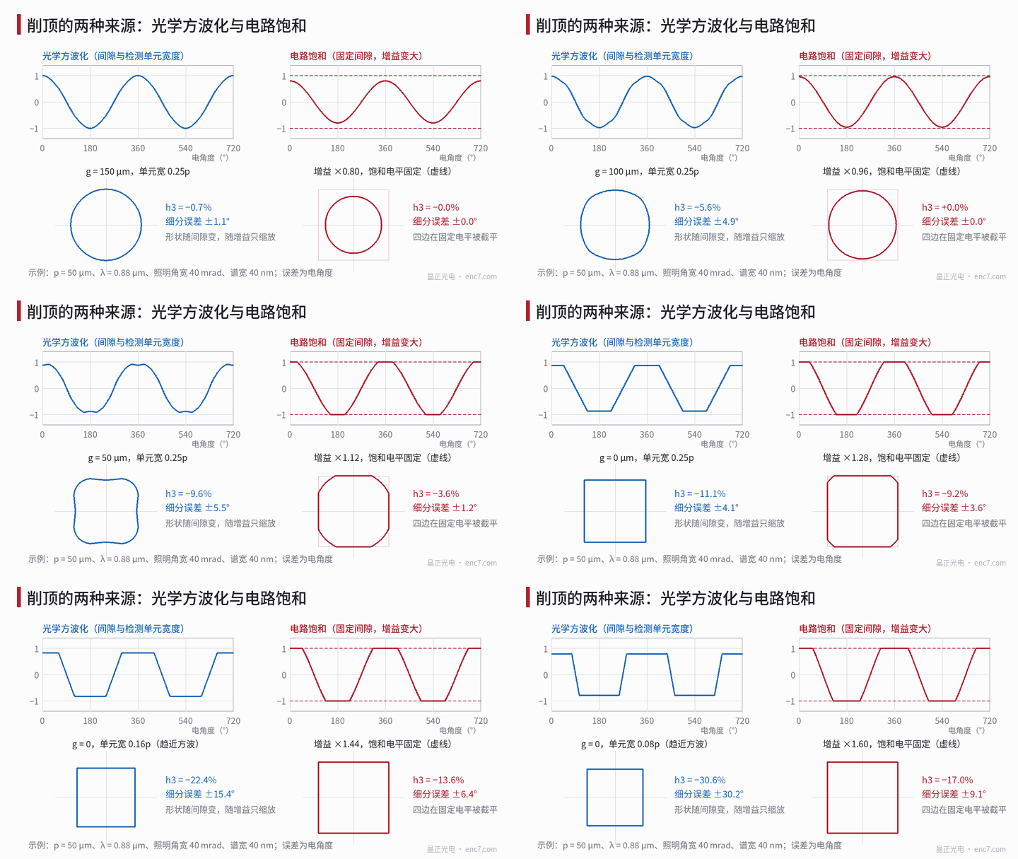
| Signature | Circuit saturation | Optical squaring |
|---|---|---|
| Flat-top level | Fixed voltage (supply rail, ADC full scale), same on all channels | Scales with amplitude |
| Junction of flat and slope | Sharp corner | Rounded, more so at larger gap |
| After reducing gain or light | Flat top disappears, sine restored | Shape unchanged, just smaller overall |
| After changing gap | Flat-top level unchanged | Waveform shape changes |
| Lissajous figure | Four sides cut by straight lines at fixed coordinates | Squircle with bulging corners, shape independent of amplitude |
One situation breaks the “fixed flat-top level” rule: saturation at a single-ended node before differential subtraction (e.g. one transimpedance output hitting the rail first). The flat top after the difference is then not at a fixed level and is often asymmetric top to bottom. When the flat top looks odd, check the single-ended test points.
Circuit saturation: harmonics and error of a clipped sine
Let c be the ratio of saturation level to sine peak, A = clip(cosθ, ±c), and likewise B. Each peak’s flat top lasts arccos(c)/π of the period. For c above 1/√2 only one channel is clipped at a time; over the clipped section the computed angle is arctan(sinθ/c), the error e(θ) = arctan(sinθ/c) − θ, reaching its maximum at
cosθ* = [−c + √(4 + 5c²)] / 2
Computed directly by atan2 (at 2,048 lines, 1° electrical is about 1.76″):
| c | Flat-top time / period | h3 | h5 | Peak interpolation error |
|---|---|---|---|---|
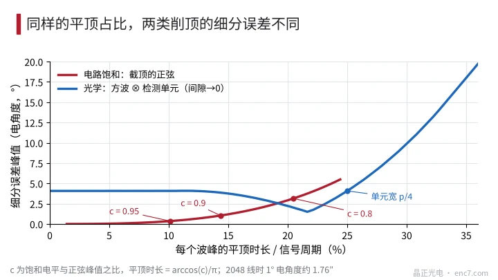
| 0.95 | 10.1% | −1.2% | −1.1% | 0.36° (0.63″) |
| 0.90 | 14.4% | −3.3% | −2.3% | 1.05° (1.84″) |
| 0.85 | 17.7% | −5.7% | −3.2% | 1.98° (3.5″) |
| 0.80 | 20.5% | −8.2% | −3.5% | 3.15° (5.5″) |
Cutting off 10% of the peak gives about 1° of error, four times per period. If only one supply rail is hit (common when the signal has an offset), even harmonics and a once-per-period error component also appear.
Optical squaring: trapezoidal waves at small gap
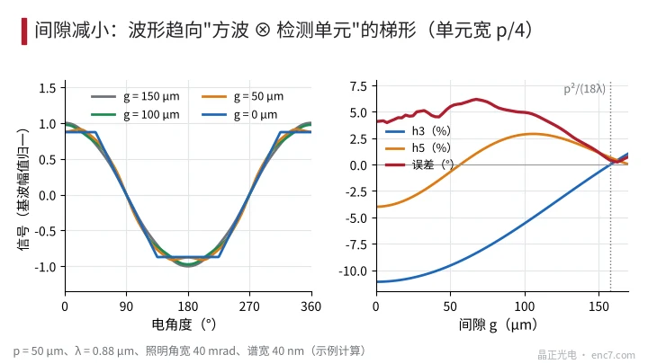
As the gap approaches zero, near-field diffraction and source blur both vanish, and the signal is simply the convolution of the disc transmittance square wave (50% duty cycle) with the detector element window. When the window width w·p is less than half a pitch, the result is a trapezoid: slope width w·p, each flat top taking 0.5 − w of the period. The p/4 element common in four-phase arrays gives a 25% flat top, h3 = −1/9, h5 = −1/25 and an interpolation error of about 4.1° (about 7.2″ at 2,048 lines); the Lissajous figure is exactly a square. Narrower elements approach a square wave: about 9.9° error at w = 0.2 and about 27° at w = 0.1. With a 50% index grating, contact gives a triangle wave rather than a trapezoid (see the next article).
As the gap increases, the nth harmonic is multiplied by the near-field factor cos(πλg·n²/p²) and a source-blur factor; higher harmonics are weakened first and the flat top gradually rounds. Example (assuming p = 50 μm, λ = 0.88 μm, element width p/4, illumination angular width 40 mrad, spectral width 40 nm):
| Gap g | h3 | h5 | Total harmonics | Interpolation error |
|---|---|---|---|---|
| 0 | −11.1% | −4.0% | 12.1% | 4.1° |
| 50 μm | −9.6% | −0.7% | 9.8% | 5.5° |
| 100 μm | −5.6% | +2.9% | 6.3% | 4.9° |
| 150 μm | −0.7% | +1.1% | 1.3% | 1.1° |
As the gap shrinks, h3 and total harmonics rise monotonically and the flat top becomes more obvious; but the error is not monotonic, because h5 changes sign along the way and the error depends on h5 − h3 (Figure 2). So “doesn’t look very flat” does not mean small error. Once the gap passes p²/(18λ) (about 158 μm here) h3 reverses sign and the waveform becomes peaked.
Comparison tests: reduce gain vs adjust gap
- Reduce gain or LED current by 20%–30%. If the flat top disappears completely and h3 returns near zero, it is circuit saturation; if h3 is essentially unchanged and the waveform just shrinks, the source is optical. This is the fastest and most reliable step.
- Look at the flat-top level and raw codes. A flat-top level exactly at the supply rail or ADC full scale, or many full-scale codes in the raw ADC data, directly identifies saturation.
- Adjust the gap. Add or remove a few tens of microns with shims (steps on the order of p²/(36λ)); an optical source’s h3 changes as in Figure 2, while the saturation type’s flat-top level stays the same, the clipped fraction changing only slightly with amplitude.
- Check single-ended nodes. When the differential output’s flat top is asymmetric or its level not fixed, measure each single-ended output to find which node saturates first.
In practice saturation mostly occurs like this: gain is set for the minimum amplitude at maximum gap with the dirtiest disc, and then a disc with a smaller gap and higher transmittance pushes amplitude over range. Size gain headroom on the maximum possible amplitude, leaving 10%–20% margin.
Estimating interpolation error from the degree of clipping
Identify the type first, then read:
- Saturation type: measure on the scope the ratio of a peak’s flat-top time t_f to the period T; c = cos(π·t_f/T), then find the error from the table above or e(θ*).
- Optical type: the flat top has rounded transitions, so timing it is unreliable; do an FFT of one channel and estimate the error from h5 − h3 (derivation in the “squircle” article).
The two relationships differ greatly (Figure 3): with a 10% flat top, saturation error is about 0.36°, while an optical trapezoid at contact gap (w = 0.4) is about 4.1°; with a 20% flat top they are about 3.1° and 2.3°. So one empirical curve cannot be used for both.
Engineering notes
- The first step is always to reduce gain or light: flat top disappears → saturation; shape unchanged → optical.
- Saturation-type error can be estimated from flat-top time, c = cos(π·t_f/T); clipping 10% of the peak (c = 0.9) gives about 1° electrical.
- Optical squaring needs two conditions: gap much smaller than p²/(18λ), and detector element narrower than half a pitch; a p/4 element at contact gives about 4.1° error.
- With an optical source, flatness changes monotonically with gap but error does not, because h5 changes sign; judge by FFT.
- When the differential output’s flat-top level is not fixed, check whether a single-ended node before the difference saturates first.
- Leave 10%–20% gain headroom on maximum amplitude; a p/3 detector element cancels the 3rd harmonic at small gap, but the 5th is still about 4%, and lower error requires gap and spatial filtering design together.
Summary
A clipped sine is either a circuit saturating at a fixed level, or, at small gap, the signal approaching the convolution of the disc square wave with the detector element. The former disappears when gain is reduced and its error converts directly from flat-top time; the latter keeps its shape with gain, changes with gap, and its error must be computed from h3 and h5. Do the gain-reduction test first to identify the type, then fix it through gain headroom or through gap and detector-element design respectively.
Translated from the ENC7 Chinese technical library (article 0228). Read the Chinese original. Need a disc built to your drawing? Request a quote or see our custom encoder discs.
© Langfang Jingzheng Optoelectronic Technology Co., Ltd. All rights reserved. This article was created with AI assistance.