Industry applications in depth
Wafer Prealigners: Notch, Eccentricity and Encoder Resolution
A prealigner turns the wafer through one revolution and uses edge readings from a line-scan sensor to fit the eccentricity and locate the notch at the same time. This article gives the eccentricity accuracy σ_c = σ·√(2/N), compares three notch-detection methods, and, for a 300 mm wafer notch of ±0.02°, derives the requirements on the encoder, the sampling rate and the synchronization.
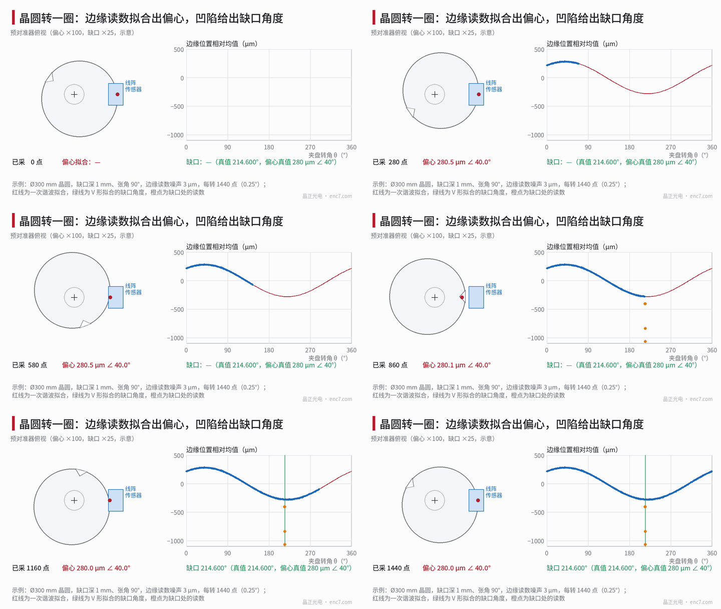
A prealigner holds the wafer on a vacuum chuck and turns it through one revolution. A line-scan sensor stands at the wafer edge and each sample yields an edge position. The data from this one revolution answer two questions at once: how far the wafer centre is offset from the chuck axis, and at which angle the notch lies. The former is obtained by fitting, the latter by finding the depression. The turntable encoder tags each sample with an angle; its line count, accuracy and synchronization determine how accurately the notch angle can be obtained.
The model: eccentricity and the notch in the edge readings
The wafer radius is R = 150 mm, the centre is offset from the chuck axis by e in the direction φ. When the chuck angle is θ, the edge position at the sensor is
r(θ) = R + e·cos(θ − φ) + n(θ) − notch
where n is the single-point reading noise (standard deviation σ, taken as 3 μm in the example) and the notch term is a V-shaped depression about 1 mm deep with an opening angle of about 90° (the SEMI standard specifies the notch dimensions for 300 mm wafers; the standard text governs). The slope of each flank is about 1, the arc length of each flank along the edge is about 1 mm, corresponding to 0.38°, and the whole notch is about 2 mm (0.76°). ±0.02° is only 52 μm on the edge. When the eccentricity is larger, the second-order term is about e²/(2R); at e = 1 mm it is 3.3 μm and can be removed by iteration.
Eccentricity: how accurately N points locate the centre
Taking N points uniformly and performing a least-squares fit of the first harmonic, the standard deviation of each eccentricity component is (the derivation is in a related article in this library)
σ_c = σ·√(2/N)
For σ = 3 μm, N = 100 gives 0.42 μm and N = 1440 gives 0.11 μm; to have σ_c ≤ 1 μm, only N ≥ 2 × 9 = 18 is needed. Noise is not the bottleneck. What must be watched is that points in the notch region are excluded from the fit, and that higher-order roundness deviations of the wafer outline can alias into the first harmonic when the number of points is insufficient.
Eccentricity also affects the notch angle: the angle of the notch relative to the wafer centre differs from the chuck angle by e/R·sin(…); at e = 280 μm the maximum is 0.107°, far larger than ±0.02°, so a correction with the fitted eccentricity is mandatory; after correction the residual is σ_c/R = 0.11 μm ÷ 150 mm, only 0.00004°.
The notch: the sampling interval decides the detection method
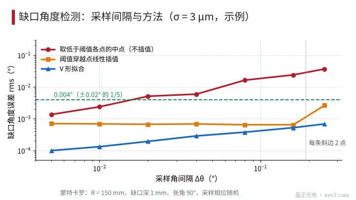
The notch angle is obtained by one of the three methods below. The relation of the error to the sampling angular interval Δθ is shown in Figure 2 (Monte Carlo, σ = 3 μm, random sampling phase):
| Δθ | Points per revolution | Sampling rate (1 r/s) | Mid-point of the points below the threshold | Interpolation of the threshold crossings | V-profile fit |
|---|---|---|---|---|---|
| 0.01° | 36 000 | 36 kHz | 0.0024° | 0.0007° | 0.0001° |
| 0.02° | 18 000 | 18 kHz | 0.0051° | 0.0007° | 0.0002° |
| 0.08° | 4 500 | 4.5 kHz | 0.016° | 0.0006° | 0.0004° |
| 0.16° | 2 250 | 2.25 kHz | 0.024° | 0.0006° | 0.0005° |
Without interpolation the error is about 0.15–0.25 times Δθ. To reach 0.004° (1/5 of ±0.02°), Δθ must be no greater than about 0.016°, which at 1 r/s is a sampling rate of about 22 kHz. The fit uses every point on the flanks: with n_f points on each flank and a slope of 1, the error of the notch centre is σ/√(2·n_f), and on the edge n_f = 0.38° ÷ Δθ. At Δθ = 0.176° (2048 points per revolution) one has n_f ≈ 2.2, and the error is 3 μm ÷ √4.4 = 1.4 μm, or 0.0006°, which agrees with the values in the table. When each flank has fewer than 2 points (Δθ greater than about 0.19°), the interpolation method fails first and the fit error also rises rapidly (Figure 2).
Worked example: how fine an encoder ±0.02° requires
Settings (example): speed 60 r/min (360°/s), 2048 points per revolution (2.05 kHz, triggered by dividing down the encoder count), V-profile fit. The encoder quantization is given a share of 0.004°, which requires not fewer than 360° ÷ 0.004° = 90 000 counts per revolution, i.e. 17 bits (0.00275°), for example 4096 lines × 32 interpolation. If only square-wave fourfold decoding is used, 4096 lines give only 16 384 counts (0.022°), which is not enough; more than 22 500 lines are needed, or a change to sine-cosine interpolation.
Synchronization: ω·Δt at 360°/s is 0.0072°/20 μs, so the jitter between sensor sampling and encoder latching must be of the order of 5 μs (0.0018°); a fixed delay is subtracted after calibration. During the exposure the edge moves at ωR = 942 mm/s; a 50 μs exposure smears 47 μm, and it is sufficient to take the timestamp at the mid-point of the exposure.
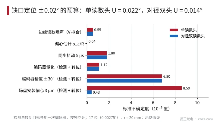
The error budget is combined as standard uncertainties. The encoder is used once to detect the notch and once to turn to the target angle, and the related terms are treated as independent and counted √2 times (encoder accuracy ±30″, disc radius r = 20 mm, eccentricity 3 μm, all example assumptions):
| Item | Single readhead | Diametrically opposed dual readheads |
|---|---|---|
| Edge-reading noise (V-profile fit) | 0.0006° | 0.0006° |
| Eccentricity estimate σ_c/R | 0.00004° | 0.00004° |
| Synchronization jitter 5 μs | 0.0018° | 0.0018° |
| Encoder quantization (17-bit) | 0.0011° | 0.0011° |
| Encoder accuracy ±30″ | 0.0068° | 0.0068° |
| Disc eccentricity 3 μm (31″) | 0.0086° | 0.0004° |
| Combined u_c / U (k = 2) | 0.0112° / 0.022° | 0.0072° / 0.014° |
With a single readhead, U = 0.022°, which exceeds ±0.02°. The main contributions are disc eccentricity and accuracy; diametrically opposed dual readheads reduce the eccentricity residual to 5%, and U falls to 0.014°. The eccentricity can also be assembled to within 1 μm, giving U of about 0.015°. Line count and sampling rate are not the difficulty here; edge noise, quantization and the eccentricity estimate together come to less than 5% of the total variance (Figure 3).
Engineering points
- First convert the specification into an angle and an arc length: ±0.02° = 72″, which on the edge at R = 150 mm is 52 μm; each notch flank is only about 0.38° wide.
- Fit the eccentricity with a least-squares first harmonic, σ_c = σ·√(2/N); a few tens of points are enough. Exclude the notch region, and correct the notch angle with the fitted eccentricity (the correction is 0.107° at e = 280 μm).
- Detect the notch with a V-profile fit or interpolation, and avoid taking only the points below the threshold: the latter requires Δθ ≤ about 0.016°, or about 22 kHz at 1 r/s.
- Give the encoder quantization 1/5 of the share, about 0.004°; 17 bits are sufficient. Square-wave fourfold decoding needs a higher line count.
- Accuracy and disc eccentricity take the larger part of the budget: use diametrically opposed dual readheads, or assemble the eccentricity to within 1 μm.
- Synchronize sampling with the encoder latch; each doubling of speed also tightens the synchronization requirement by the same factor; take the exposure timestamp at the mid-point.
In brief
On a prealigner the eccentricity is obtained by a first-harmonic fit, σ_c = σ·√(2/N), and a few tens of points are enough; the notch is obtained by a V-profile fit or interpolation, and a sampling rate of the order of 2 kHz is sufficient. For a 300 mm wafer notch specified at ±0.02°, a 17-bit encoder, 2048 points per revolution and 5 μs synchronization are enough. What really has to be controlled is the encoder accuracy and the disc eccentricity; diametrically opposed dual readheads are the most direct method.
Translated from the ENC7 Chinese technical library (article 0770). Read the Chinese original. Need a disc built to your drawing? Request a quote or see our custom encoder discs.
© Langfang Jingzheng Optoelectronic Technology Co., Ltd. All rights reserved. This article was created with AI assistance.