Industry applications in depth
Wafer Robots: ±0.1 mm Placement Repeatability and Joint Encoders
At a placement repeatability of ±0.1 mm and a reach of 700 mm, the total angular budget of the θ-axis is only 29.5″. Starting from example figures, this article subtracts the reducer and structural errors, arrives at about 10″ for the encoder-related terms, compares a motor-side arrangement with an output-end arrangement, and estimates an upper bound on adhesive outgassing in a cleanroom (about 1.4 nm for 0.1 g).
A wafer-handling robot carries 300 mm wafers from the cassette to the process chamber, and the placement-position repeatability is often quoted as ±0.1 mm. The joint is at the centre and the wafer is at the end of the arm, so an angular error of the θ-axis is magnified by the reach into a position deviation. The placement specification must therefore first be converted into an angular budget before encoder requirements can be stated.
From ±0.1 mm to an angular budget
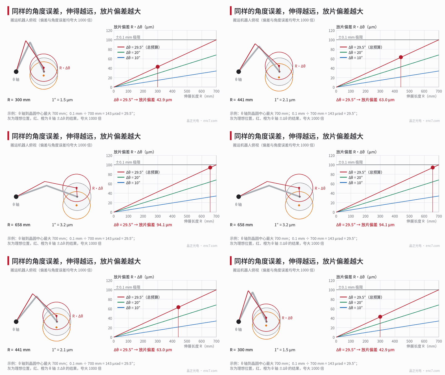
The θ-axis rotates the entire arm about the axis, and the tangential deviation of the wafer centre = R·Δθ. In the example the maximum distance from the θ-axis to the wafer centre is taken as R = 700 mm, so
1″ = 700 mm × 4.848×10⁻⁶ = 3.39 μm,0.1 mm ÷ 700 mm = 143 μrad = 29.5″
This is the budget for all causes combined. The shorter the extension, the smaller the position error for the same angular error: at R = 300 mm, 29.5″ is only 43 μm, so the maximum reach is the one that governs. If the ±0.1 mm specification is given as 3σ, then σ is about 9.8″, and every term below should be understood with the same statistical meaning.
Subtracting reducer and structural errors
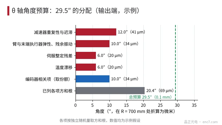
Not all of the θ-axis deviation belongs to the encoder. The following are example assumptions (angles at the output end, independent random quantities combined by root-sum-square):
| Item | Angle | At 700 mm |
|---|---|---|
| Reducer repeatability and hysteresis | 12″ | 41 μm |
| Arm and end-effector elasticity, residual vibration | 10″ | 34 μm |
| Servo settling residual | 6″ | 20 μm |
| Temperature drift | 6″ | 20 μm |
| Root-sum-square | 17.8″ | 60 μm |
From √(29.5² − 17.8²) = 23.5″, at most 23.5″ is left for the encoder-related terms. Leaving a margin for unlisted items (wafer slip on the pad, coupling from the radial axes, and so on), the encoder is given 10″; the combination is 20.4″ (69 μm), and 21″ still remains (Figure 2).
Encoder arrangement: motor side or output end
The resolution is taken as q ≤ 1/5 of the share: 10″ ÷ 5 = 2″, so at least 648 000 counts per revolution (about 19.3 bits). Taking 2²⁰ (4096 lines × 256 interpolation) gives 1.24″ per count.
| Arrangement | Encoder-related terms (output end) | Notes |
|---|---|---|
| Motor side, reduction ratio 50, 17-bit (9.9″) | quantization 0.2″, accuracy ±60″ referred 1.2″ | the encoder itself is barely a limitation, but it cannot see the reducer’s 12″ |
| Hollow encoder disc at the output end, single readhead | eccentricity of 3 μm at r = 60 mm is 10.3″ | already exceeds the 10″ share |
| Hollow encoder disc at the output end, diametrically opposed dual heads | eccentricity residual of 5% is 0.5″, U ≈ 5.9″ | satisfies the budget |
Combination for the diametrically opposed dual-head arrangement: accuracy ±5″ (2.9″), eccentricity residual 0.5″, quantization 1.24″ ÷ √12 = 0.36″, interpolation error from a 1% signal offset 316″ × 0.01 ÷ 2π = 0.5″ (taking amplitude ÷ √2 gives 0.36″), noise 0.3″, u_c = 3.0″, U (k = 2) about 6″, less than 10″. When the reduction ratio is large and the reducer itself is accurate, a motor-side encoder is sufficient; with direct drive, or when reducer error is to be compensated inside the loop, the encoder disc should be mounted at the output end.
Clean environment: particles, materials and outgassing
Material outgassing in vacuum is already covered by a dedicated article in this library; only an atmospheric cleanroom is considered here.
Particles. An optical encoder reads without contact, so there is no wear between the encoder disc and the readhead. Residual sources are edge chipping of the disc, adhesive squeeze-out or crumbs, cable jackets, and dust that enters during assembly. Disc edges should be chamfered and polished, and finished cleanliness should be accepted against the grade curves in this library; glass is insulating and readily becomes electrostatically charged, and the problem of particle attraction is the subject of another dedicated article in this library. A common practice is to keep a negative-pressure exhaust inside the robot so that particles do not drift toward the wafer side.
Materials. A glass substrate with a chrome layer has low outgassing and very little moisture uptake; plastic substrates generally take up more moisture and outgas more, and must be assessed item by item. For bonding and sealing, use a low-outgassing adhesive as far as possible, and restrict siloxane-containing materials, which are often tightly controlled in a semiconductor environment.
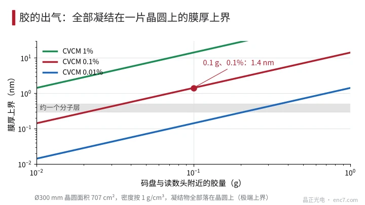
Outgassing. Organic volatiles released by the adhesive can condense on the wafer. A commonly used screening line is a total mass loss TML ≤ 1% and collected volatile condensable material CVCM ≤ 0.1% (the ASTM E595 test conditions are vacuum, 125 °C and 24 h, which are more severe than a cleanroom; whether they apply is determined by the user’s specification). Example: 0.1 g of adhesive is present near the encoder disc, and CVCM is taken as 0.1%, i.e. 0.1 mg; if it all condenses on a Ø300 mm wafer (area 707 cm²), and the density is taken as 1 g/cm³, the film thickness = 0.1 mg ÷ 707 cm² ÷ 1 g/cm³ ≈ 1.4 nm (Figure 3). This is an extreme upper bound; in reality only a small fraction reaches the wafer, but it already shows the order of magnitude: the amount of adhesive must be small, cure and bake-out must be thorough, and whether the result is acceptable depends on the process.
Engineering points
- First convert the placement specification into an angle with R·Δθ: at 700 mm, 1″ = 3.39 μm, and ±0.1 mm is 29.5″; evaluate at the maximum reach.
- Subtract the reducer, structure, servo and thermal drift first, and give the encoder-related terms a share (10″ in the example); do not give the entire budget to the encoder.
- Take the resolution at no more than 1/5 of the share, about 2″; an encoder with 2²⁰ counts is sufficient.
- With a single readhead, eccentricity is the largest term; use diametrically opposed dual readheads on a large-diameter encoder disc at the output end, and also check the interpolation error caused by signal offset.
- When the reduction ratio is large and the reducer is stable, choose a motor-side encoder; when reducer error is to be compensated inside the loop, choose an output-end encoder disc.
- In a cleanroom the priorities are outgassing and particles: a low-outgassing adhesive, a small amount of adhesive, chamfered edges, clean packaging, and internal exhaust kept in operation.
In brief
A placement repeatability of ±0.1 mm at a 700 mm reach corresponds to a total θ-axis budget of 29.5″. The reducer and the structure first take the larger part; about 10″ is enough for the encoder-related terms, and 2²⁰ counts with diametrically opposed dual readheads will do. The extra cleanroom requirements are on the materials: a glass substrate with a chrome layer, a low-outgassing adhesive, a small amount of adhesive, and reliable exhaust, so that the condensed volatiles from the adhesive stay within what the process can accept.
Translated from the ENC7 Chinese technical library (article 0769). Read the Chinese original. Need a disc built to your drawing? Request a quote or see our custom encoder discs.
© Langfang Jingzheng Optoelectronic Technology Co., Ltd. All rights reserved. This article was created with AI assistance.